April 18, 2005 marks the 10th anniversary of The Michigan Economic Growth Authority, a program established by Michigan government with the mission of spurring in-state job creation and business investment. The authority is the state of Michigan’s agent for selecting firms to receive Single Business Tax credits in return for creating new facilities and jobs in Michigan.
April 18, 2005 marks the 10th anniversary of The Michigan Economic Growth Authority, a program established by Michigan government with the mission of spurring in-state job creation and business investment. The authority is the state of Michigan’s agent for selecting firms to receive Single Business Tax credits in return for creating new facilities and jobs in Michigan. These MEGA agreements also result in local incentives for the recipient firms, and often in other state incentives, as well.
MEGA was originally limited to providing packages only to firms that created new jobs at single sites in such industries as manufacturing, office operations, or research and development. Five substantive amendments to the program since 1995 have allowed MEGA to offer packages in return for smaller job and investment totals, for the retention of existing jobs, and for jobs in additional industries.
Through 2004, more than $1.8 billion in Single Business Tax relief has been offered to more than 200 firms in 230 MEGA agreements over as much as 20 years. The value of these MEGA agreements rises to more than $3 billion with the inclusion of other state and local incentives, such as property tax abatements, job training subsidies and infrastructure improvements. Nearly one-third of this total — $987 million — has been provided by local units of government or by local economic development agencies.
Scholarly estimates suggest that nationwide, the targeted incentives distributed by state and local governments exceed $50 billion annually.
The number of MEGA packages and the total size of the SBT credits offered each year has generally been rising, despite dips in 1997, 2001 and 2003. In 1996, MEGA’s first full year, MEGA offered just 15 deals, totaling $89.9 million in SBT credits. In 2004, however, MEGA produced 41 packages valued at $253.3 million (for up to 20 years) in SBT relief alone.
Direct Jobs
MEGA agreements are expected to create two types of jobs — "direct" and "indirect." "Direct" jobs are new jobs at the specific firm sites that are the subject of the MEGA package. "Indirect jobs" are new jobs created outside these specific firm sites in response to MEGA-related investment and direct employment.
State documents indicate that approximately 127 of MEGA’s agreements should have produced fully employed facilities through 2004 — i.e., sites hosting all of their projected direct jobs.
Of these 127, about 56, or 44 percent, have claimed credits under the MEGA program. A company can claim these tax credits, however, without meeting the initial total direct job projections.
In fact, only about 10 of these 56 cases can be shown to have created the number of direct jobs originally projected within the expected time frame.
MEGA originally projected that these 127 MEGA deals would generate 35,821 direct jobs by 2005. MEGA figures obtained in December 2004 shows that these deals have actually generated about 13,541 direct jobs — roughly 38 percent of original expectations.
MEGA’s direct job total through late last year thus represents about 0.3 percent of Michigan’s 2004 workforce.
Between 1996 and 2004, MEGA originally estimated that more than $220 million in SBT credits would be redeemed as a result of MEGA agreements. Lagging direct job creation, however, meant that companies claimed just $75 million in credits, or about 34 percent of original expectations.
Indirect Jobs
In two commentaries published in newspapers in November 2004, state officials claimed that the MEGA program had produced 28,812 total jobs. This figure is higher than 13,541 because it includes indirect jobs purportedly created by the program.
MEGA’s estimate of the indirect jobs in the 28,812 job total is unreliable for at least four reasons:
It employs a constant, rather than a varying, formula for MEGA’s diverse projects, even though MEGA’s own analyses show that these projects have different potentials for generating indirect jobs;
It implicitly employs assumptions about the economy in future years — well past 2005 — in order to estimate indirect jobs for past years;
It implicitly counts indirect jobs that would be created only after 2005 in its indirect job estimates for the past 10 years, thereby overstating the numbers;
It fails to fully correct assumptions made in earlier years that have since proved too optimistic, with the likely result of overstating the numbers.
Because MEGA could theoretically generate economic benefits despite its lagging success rate, the authors employed a detailed econometric analysis to determine whether MEGA credits influenced economic growth in Michigan counties during the years 1995 to 2002 (2002 was the last year for which county-level data are available). The authors also tested the impact of MEGA credits on the manufacturing, warehousing and construction sectors. The authors found the following:
MEGA did not improve Michigan’s per-capita personal income, employment or unemployment rate.
MEGA did not improve any Michigan county’s per-capita personal income, employment or unemployment rate (estimates of impact ranged from zero to modestly, though not significantly, negative);
Michigan counties that did not host companies receiving MEGA deals fared as well as counties that did host such companies;
MEGA essentially did not affect aggregate income or employment in manufacturing and warehousing (the one statistically significant effect was negative, but too small to be economically significant);
MEGA apparently caused a temporary shift to higher construction employment without increasing overall employment. One temporary construction job was created for every $123,000 in MEGA credits awarded; 75 percent of these jobs disappeared after one year, and the remaining 25 percent fell away after two. There was a concurrent, statistically significant decline in construction wages as a result of MEGA credits, but it was too small to be economically meaningful.
There are potentially several reasons why MEGA’s actual economic impact has been less than expected, as is shown by a review of specific MEGA projects, the academic economic literature and information about MEGA’s procedures. These reasons fall into four categories:
Political and Business Incentives Can Interfere With MEGA’s Policy Goals
Academic economic literature increasingly recognizes a "political economy" in public policy whereby political incentives to gain public approval for a program and its supporters can interfere with effective policy decisions. In economic development programs, this dynamic can favor projects with a higher public profile, such as those that benefit well-known or exciting new businesses or industries, even if these efforts are not necessarily the wisest use of resources.
State officials’ promotion of MEGA and other state economic development programs has in the past suggested political incentives may be playing a role in officials’ support for these policies. Legislative support for the Jobs I and Jobs II packages in 2003 appear to be instances of this.
Concern over potential political appeal may also be evident in several apparent overestimates of job impact by state officials in MEGA and related state programs. In one specific MEGA agreement, a company official detailed his disagreement with MEGA’s projections of job creation at his firm. Michigan’s auditor general has also twice criticized (non-MEGA) Michigan development agencies for the overstated job creation numbers the agencies had reported on audited programs.
Such overestimates of economic impact are not particular to Michigan. A Toledo, Ohio-area economic development agency recently reduced its own job creation claims substantially following the departure of an agency executive. Media scrutiny played a role in this reduction, but it came several years after the fact, and after the responsible official had departed — a delay in accountability that is unsurprising given the long-term nature of economic development programs.
The presence of targeted economic development programs can generate counterproductive business incentives, as well. A recent study of the state of Ohio’s economic development incentives between 1993 and 1995 found that while the incentives had no positive economic impact, the businesses that received incentives were more likely to overestimate employment forecasts than businesses that had not. Similarly, at least one major consulting firm has recently counseled businesses on how to position themselves aggressively to receive state economic development grants. Such tactics can lead government officials to favor less productive deals over better ones.
The MEGA program could begin to serve specific, short-term political and corporate interests, rather than the long-term goals that inspired the program. Not only might this combination of interests lead to a misallocation of state development monies toward less effective projects; it might also lead to lower economic growth, according to a 1999 study of state economic statistics in the continental United States.
The Inherent Complexity of the Marketplace
MEGA officials are faced with the task of picking companies that can create and sustain jobs in the Michigan marketplace. But the marketplace decisions that lead to new employment and new business investment in Michigan are made by millions of individuals with their own subjective preferences and individual understanding of local market conditions. The economic literature increasingly recognizes that the inherently dispersed nature of their knowledge and preferences makes predictions about which companies can successfully create and maintain new jobs exceedingly difficult for any observer or organization to determine. One recent analysis shows that that between 1995 and 2000, only one of the 45 largest stock funds outperformed the Standard and Poor’s 500 index, and it did so only by a small margin.
Assumptions in the "REMI" Modeling Employed by MEGA
MEGA engages economists at the University of Michigan to aid MEGA’s future employment projections through the use of a respected computer-based economic model known as REMI, short for Regional Economic Modeling Inc. The REMI modelers at the university appear to use the model skillfully and responsibly.
Nevertheless, several aspects of the model and the assumptions used with it may be leading to optimistic estimates. These issues involve the treatment of the direct cost of state tax relief, the cost of local incentives in MEGA packages, the differences between high- and low-unemployment areas, the failed employment and wage assumptions apparent in past simulations, and the potentially increased cost of new state and local government services following new business investment and employment.
The Problem of Ensuring MEGA Credits Are Necessary
State law specifically requires MEGA to determine that "the expansion or location of the eligible business will not occur in this state without the tax credits offered under this act." If there is an error in determining this — i.e., if a firm would have located in Michigan without the credit — the cost of the credit to the state and its economy rises.
In practice, making such a determination will be difficult, both for MEGA officials and for the firms concerned. Several case studies indicate how business calculations can change, so that an unattractive location may become attractive on further review, despite the absence of a tax credit. The potential for a revision of opinion can be particularly high if a firm already had strong reasons to locate in a particular location.
One way to determine the rate at which businesses might not ultimately need a credit that initially appears essential would be to study the subsequent actions of businesses that sought MEGA credits but were denied them. Gathering a comprehensive list of such firms has proved difficult, however.
End the MEGA Program
Given the underperformance of MEGA projects, the program’s manifest lack of economic impact in its first seven years, and the inherent difficulties in making such a program work, it would probably be best to cancel the MEGA program. The state has alternative ways to improve its business climate that are more likely to be effective.
Concerns about MEGA are only amplified by questions about the program’s fairness to firms that do not receive tax credits. These concerns are further underscored by a recent federal court case that suggests MEGA may be unconstitutional.
Other Reforms
While reforms of the MEGA program are unlikely to increase its economic value, policy-makers can take several steps that might improve MEGA if they choose to continue it:
Audit MEGA. The state could consider asking the Office of the State Auditor General to conduct regular, expanded audits of MEGA’s direct job counts. Such oversight could help improve the authority’s accounting procedures. The auditor general’s office could also be encouraged specifically to review applications by MEGA candidates that were rejected. The results of such a review could help clarify the extent to which the MEGA credits have truly been necessary.
Count Direct Jobs Only. It would probably facilitate public review and understanding of the MEGA program if indirect job benefits were no longer reported and cited by MEGA officials. "Spin-off" considerations could still be part of the evaluation process for a particular project, but MEGA would no longer make a formal or informal practice of tallying the indirect jobs its past and future projects could claim. Removing MEGA officials’ focus on indirect job counts might free the authority to more carefully document its direct job creation.
Develop a Transparent Framework for Tracking Success and Failure. The status of each MEGA project could be posted and updated live on the Web each month to show such basic items as the following: the state and local incentives offered in each MEGA package; the state and local incentives claimed in each MEGA package; the cost of these incentives so far and in the current year; the current direct job figures; what the direct job figures were originally projected to be at present; and so on. Such reporting would facilitate effective public oversight of the program’s effectiveness.
Commission an Independent Econometric Review. An independent researcher could be engaged to maintain a peer-reviewed and publicly transparent econometric model that annually reassessed MEGA’s impact. The model employed in this study was crafted to detect past impact, rather than predict future performance. Regular updates of the findings would therefore be appropriate if the MEGA program continues.
In recent decades, the age-old economic competition among the United States has turned into an economic battle for specific companies and jobs. It is a skirmish fought with targeted tax incentives, such as abatements in property or business taxes, offered to firms seen by government officials as particularly desirable for their ability to create jobs and stimulate broader economic growth.
Kenneth Thomas, a University of Missouri-St. Louis political scientist, estimates that the cost of U.S. state and local incentives provided to corporations every year is $48.8 billion in 1996 dollars[1] (though his figure excludes incentives offered in Kentucky, due to a dearth of data). Thomas is not the only scholar to tally a figure of this magnitude. University of Iowa economists Peter S. Fisher and Alan H. Peters believe the annual value of state and local incentives distributed in pursuit of “economic development” exceeds $50 billion.[2]
The Michigan Economic Growth Authority is Michigan’s primary tax incentive program. Established by former Gov. John Engler and the Michigan Legislature in the hope of fostering state job growth by encouraging specific out-of-state businesses to relocate to Michigan and specific Michigan businesses to expand here, the program’s 10th birthday is April 18, 2005.
State documents show that in the past 10 years, MEGA has offered business tax relief exceeding $1.8 billion to more than 200 companies in a total of 230 deals (the exact number of companies depends on how one counts subsidiaries and acquisitions).[3] This is a substantial track record. It allows us to form meaningful conclusions about the program’s effectiveness as an instrument for stimulating Michigan’s economy.
As we recount in "Appendix E: A Brief History of State Economic Development," there have been at least eight major institutional vehicles created since 1947 to carry out Michigan’s government economic development policies. These policies generally aim to improve the state’s economy by creating or retaining jobs either with specific companies or with specific kinds of companies, typically in order to promote diversification of the state’s economy away from the automobile industry. MEGA is currently the most prominent of the state’s economic development programs.
The creation of MEGA was particularly notable because of its primary champion, former Gov. John Engler. In the 1980s, Engler, then Michigan senate majority leader, had often criticized central economic "planning," chiding Gov. James Blanchard for such programs as the Michigan Strategic Fund, which was an earlier tool of state economic development planning. Engler argued that such programs were unfair because they failed to "treat everyone in the marketplace … equitably by dealing with Michigan’s oppressive tax burdens," and because such programs benefit a firm "if you are a friend of government, if you’re a friend of the current administration, if you know somebody … or any other number of keys that sort of unlock the magic door that controls these funds."[4]
When he came to office, Gov. Engler initially called for an end to state economic incentives. In February 1992, according to the Detroit Free Press, he and Gov. Jim Edgar of Illinois began trying to persuade their counterparts in other states to stop trying to lure each others’ commercial enterprises with targeted tax incentives. Engler reiterated his views at the August 1992 National Governors Association conference in Princeton, N.J., leading the Free Press to observe:
Engler believes — and he is backed by some economists — that such competition is bad in the long run because it creates an unfair tax system that often produces fewer jobs than promised. States, Engler said, should lure new businesses with good schools, low taxes and skilled workers — things that benefit all types of commerce.[5]
In keeping with these observations, Gov. Engler did implement a number of general policy changes meant to improve Michigan’s services and business climate, including tax cuts, privatization and public school choice measures. Nevertheless, following his unsuccessful attempts to persuade other governors to forgo targeted tax incentives and business subsidies, he chose to increase Michigan’s own targeted economic incentives — first, with his 1993 reorganization[6] of the state’s existing economic development programs, and second, with the introduction of MEGA, which offered targeted tax relief and other incentives to businesses to encourage them to invest or locate in Michigan.
The original MEGA law, passed in 1995, established the Michigan Economic Growth Authority as an eight-member state board that was directed by the chief executive officer of the then-Michigan Jobs Commission. This board administered the MEGA program, which provided Single Business Tax credits to corporations it chose following certain general criteria described below.[7]
MEGA’s agreements with targeted businesses required (and continue to require) a contribution to the overall MEGA incentive package from the local government or local economic development unit in the area hosting the new or expanded business facility.[8] These local business incentives usually take the form of tax abatements on real or personal property, though they sometimes include such items as permit waivers, road improvements and even discounted access to the local municipal golf course for the business’s employees.
The MEGA incentive package also can include state incentives other than Single Business Tax credits. The incentives, such as job training subsidies, were originally arranged by the Michigan Jobs Commission; later, they were provided by the Michigan Economic Development Corporation, an offshoot of the Jobs Commission that was established in 1999 to oversee the state’s primary economic development programs — including, in effect, MEGA as well.
The original law was relatively strict about who could qualify for MEGA credits. A business pursuing MEGA credits had to assure the state that it would in fact create new jobs at the specified Michigan site after the company’s executives signed the MEGA agreement. These jobs, in turn, had to involve such industries as manufacturing, research and development, or office operations. Retailing operations, such as a local Home Depot store, and tourist-related industries, such as hotels or restaurants, were excluded from assistance in the program.
The original law also required a MEGA recipient to meet relatively strict qualifications (most of these original qualifications remain despite subsequent amendments to MEGA law). As outlined in the Mackinac Center for Public Policy’s study "MEGA Industrial Policy: An Analysis of the Proposed Michigan Economic Growth Authority," the requirements included the following:
The business must create a minimum of 75 "qualified new jobs" if expanding in Michigan, or 150 qualified new jobs if locating in Michigan, within 12 months of opening the facility. A "qualified new job" means a full time job in excess of the number of jobs existing in the year before the new facility opens.
The business must agree to maintain the 75 (or 150) new jobs each year that a credit is received.
The business must agree to maintain a number of employees greater than the number employed in the year before the new facility is opened.
The average wage paid for the new jobs must be greater than the average wage paid by private-sector firms in that county.
The business must certify that the expansion or location would not have occurred in Michigan without the tax credit.
Local government must make a financial or economic commitment to the business for the facility.
The business must not have begun construction or announced the specific location of the facility.
It is the MEGA board’s job to determine if the proposed business facility or expansion meets the criteria above, as well as the following:
The expansion or location will "benefit the people of this state by increasing opportunities for employment and by strengthening the economy of this state."
The tax credit is needed due to a significant cost disparity — including economic incentives offered by a competing state — between this state and the competing state.
The business has a sound financial record based on the financial statements of the last three years.
The final step is for the MEGA board and the business to execute a written agreement that officially makes the business an "authorized business" (that is) able to receive an SBT credit. The MEGA board determines the length of the credits (not to exceed 20 years). This agreement must provide that a misrepresentation in the application or a violation of the agreement may result in revocation of the "authorized business" status and loss of the tax credit.[9]
Since 1995, the MEGA law has been substantively amended five times. Three major aspects of these changes follow, and they remain in effect today:
The MEGA program’s "flexibility"[10] was enhanced, allowing additional kinds of businesses to participate with lower job and capital investment thresholds. Such changes increased the number of MEGA deals.
MEGA law now allows the board to hand out targeted relief to a business for retaining jobs that already exist, instead of creating new ones. It also allowed MEGA credits for "high tech," "rural," and "distressed" businesses, which do not have to create as many new jobs as were originally required under MEGA law.
MEGA law now allows certain approved companies to meet their job goals by counting the total number of jobs at multiple company sites, rather than just a single facility. The state also loosened minimum capital investment and aggregate job counts for multi-site facilities.
MEGA LAW
The following is a list of amendments that made substantive changes to the original Michigan Economic Growth Authority Act of 1995. This summary highlights the major modifications; not every change to the law appears in the text below.
This legislation expanded the MEGA law to include "high-technology" businesses. Authorized high-technology businesses were required to create both a minimum of five new qualified jobs at a particular facility and 25 more within five years — a departure from the original law’s requirement that 75 new jobs be created if the business was expanding in the state. High-technology businesses receiving MEGA packages also had to agree that "not less than 25 percent of the total operating expenses of the business will be maintained for research and development for the first 3 years of the written agreement."[11] No more than 50 high-technology MEGA deals were permitted in any given year.
The act also expanded to "make the retention of jobs and businesses a goal of MEGA SBT credits,"[12] meaning the MEGA program was no longer limited simply to the creation of new jobs. Companies qualified for "retention credits" by keeping at least 500 existing jobs in the state and making at least a $250 million capital investment in Michigan.[13]
Effective Jan. 9, 2001, this legislation changed the definition of the kind of "qualified new job" that could qualify for MEGA incentives. The original law’s definition required that jobs created by the authorized business be counted as a new job only after the expansion or location occurred in Michigan. The liberalization of MEGA’s "qualified new job" definition meant that a qualified new job also included a "full-time job at a facility created by an eligible business that is in excess of the number of full-time jobs maintained by that eligible business in the state 120 days before the business becomes an authorized business, as determined by (MEGA)."[14]
This legislation dramatically expanded the number and types of businesses that could qualify for MEGA deals. For instance, the bill allowed a retention credit for businesses that "made a capital investment of $100 million between three years before and two years after becoming an authorized business and agreed to maintain at least (1,500) jobs at the facility. …" The new law also stipulated that "the (retention) credit available under this provision could be granted only as part of a package of incentives that addressed international competition and included a negotiated labor contribution," such as a wage concession.[15]
Public Act 248 also expanded MEGA to include two new types of businesses, according to the following guidelines:
Distressed businesses. A business was deemed distressed if all three of the following criteria were met:
"four years immediately preceding the application to the authority under this act, the business had 150 or more full-time jobs in this state";
"within the immediately preceding 4 years, there has been a reduction of not less than 30 percent of the number of full-time jobs in this state during the three-year period"; and
the business "is not a seasonal employer." The law also limited MEGA to executing no more than 20 new deals or less for distressed businesses each year.[16]
Rural businesses. If a business were located in an area considered "rural" — a county of 75,000 people or fewer — it could qualify for MEGA deals provided it could create five qualified new jobs at an expanded or relocated facility and maintain 25 jobs within 5 years after the expansion or relocation. This requirement was similar to those for high-technology firms. Under the law, only five new rural deals could be approved annually.[17]
This legislation expanded MEGA law to allow businesses with multiple sites in the state to receive tax credits for retained or new jobs using employment totals from more than one facility. The legislation mandated that a company with multi-site authorization not only maintain 150 retained jobs at a particular location, but maintain 1,000 or more full-time jobs across Michigan and make new capital investment in the state.[18] The legislation also included four other ways for firms to qualify for MEGA approval.
This legislation again expanded MEGA law, providing more opportunities for companies to become an authorized business. For example, the law allowed a company to qualify for MEGA deals if it retained just 100 jobs at a single facility and agreed to make a capital investment of either $10 million or $100,000 per job retained at a particular facility, whichever was greater.[19]
The primary sources of financial data concerning MEGA and its related local incentives are documents produced by the MEDC and its predecessor agency, the Michigan Jobs Commission, obtained by the Mackinac Center under Michigan’s Freedom of Information Act. Graphics 2 and 3 (see links below) provide two-page samples of the "All MEGA Projects" and "MEGA Credits" spreadsheets that are referenced throughout this study.[20]
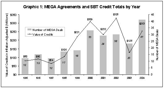
Since its inception, MEGA has offered targeted business tax relief exceeding $1.8 billion in a total of 230 deals to more than 200 companies or related subsidiaries.[21] (As mentioned earlier, the precise count of the companies involved in these deals can be debated, depending on how one treats acquisitions, subsidiaries or suppliers.[22]) Graphic 1 shows a year-by-year breakdown of total MEGA deals and the approximate, inflation-adjusted value of their respective MEGA credits.
The number of MEGA packages and the total size of the SBT credits offered each year has generally been rising, despite dips in 1997, 2001 and 2003. In 1996, MEGA’s first full year, MEGA offered just 15 deals, totaling $89.9 million in SBT credits;[23] only 25 MEGA deals were allowed annually at the time.[24] In 2004, however, MEGA produced 41 packages valued at $253.3 million (for up to 20 years) in SBT relief alone.[25]
The amount of MEGA state tax credits for individual firms has varied over the years, from a tiny offer of $160,000 to Integrity Design Inc. in April 2001 to an $88 million MEGA "retention" credit to the Ford Motor Company in November 2000 (these credits could be earned over five and 20 years, respectively).[26]
Each MEGA deal has included additional state or local tax incentives for the recipient firms. To date more than $987 million[27] has been offered to MEGA companies by local units of government or local economic development agencies. As mentioned earlier, local incentives offered in MEGA deals usually involve tax abatements on real or personal property, permit waivers, road improvements or municipal perquisites for company employees.
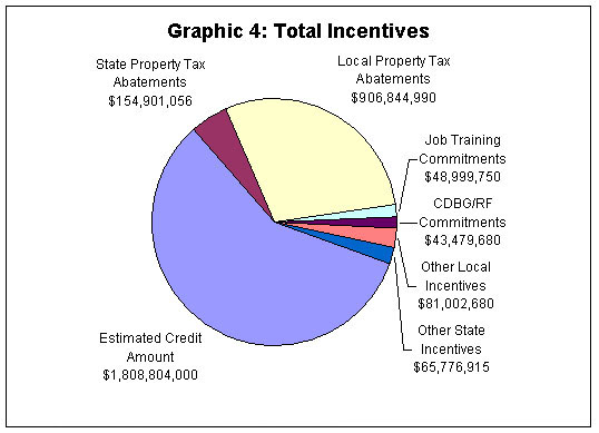
The incentives offered through MEGA packages total more than $3 billion since the beginning of the program. These incentives include state tax credits, local abatements and other state and local inducements, such as job training and road improvements. Graphic 4 shows the approximate value of all known incentives offered to recipients of MEGA deals by category.
According to MEGA Briefing Memos produced by the MEDC, the smallest local incentive in MEGA history appears to be a $28,000 break to Universal Forest Products in 2002 (though it is possible that a smaller incentive was offered that was not discernible in the MEDC documents obtained by the authors).[28] The largest local incentive was $165 million over 25 years to General Motors Corp. in June 2000.[29]
General Motors Corp. has been the direct beneficiary of six MEGA deals, by far the most of any corporation.[30] Additional MEGA deals have been concluded with GM suppliers as part of an overall package benefiting GM. For instance, CMI‑Schneible Co., Machining Enterprises Inc. and Michigan Production Machining Inc. have all received MEGA deals. The MEGA credits and other incentives offered to these companies were all designed to support the "General Motors Nodular Iron Redevelopment Project" in Saginaw.[31]
Assumptions
While calculations about jobs creation are, in theory, straightforward, they depend on assumptions that may differ. MEDC has not provided all of the clarifications we had originally sought about the basis of some of the projected MEGA jobs figures,[32] so we adopted two key assumptions: first, that all predictions of direct job creation by MEGA corporations by a certain year (1999, for example) meant the jobs would exist at midnight on Dec. 31 of the previous year (1998); second, that this previous year roughly corresponded to the tax year listed on the "MEGA Credits" spreadsheet. Changing the methodology would change the precise totals, though probably with no significant impact on the findings.[33]
Another issue that must be decided in reviewing MEGA’s performance involves distinguishing between "direct" and "indirect" jobs purportedly created by the program. The MEDC defines "direct jobs" attributable to a MEGA package as the increase in the number of jobs at the specific firm sites that are the subject of the MEGA package. It defines "indirect jobs" as those jobs that are created outside the specific MEGA business sites following the MEGA-related investment and direct employment.
We have chosen to work primarily with direct job counts in this study. Estimating indirect job counts is a subjective exercise, and econometricians and accountants with the best of intentions can produce widely varying figures, depending on their assumptions and estimation techniques. In addition, the indirect job totals implicitly claimed by state officials in recent press commentaries are, at best, rule-of-thumb estimates, and they appear to be unreliable, as we will detail below.[34] Thus, when we do discuss indirect job counts (also known as "spin-off" jobs), we will say so specifically.
Another key issue in evaluating MEGA’s track record on jobs is captured by the remarks of David Hollister, Director of the former Michigan Department of Consumer and Industry Services, in discussing MEGA’s job program:
There is usually a lag time of several years between MEGA board approval of a project and reporting of jobs created. Many of these projects involve the construction of new plants and facilities, which can take several years. Therefore the number of jobs created by MEGA-aided projects … is only a fraction of the actual number of jobs that MEGA will eventually help to stimulate. … MEGA has been in existence for less than eight years, (so) we are just beginning to see the benefits of credits granted early on.[35]
It is true that economic and financial investments can involve lag time. Thus, it is necessary to factor in the delays projected by MEGA officials in each specific tax credit package, and we have done so in our calculations in the following section. We do not assume, however, that time lags can effectively be infinite.
Finally, we would note here that we have kept track of MEDC incentives differently than MEDC officials do. MEGA officials often remove data from their "All MEGA Projects" spreadsheet for deals that fail early on, and MEGA then subtracts from the spreadsheet the amount of the incentives originally offered to those firms. We have maintained this data, so we often report different and higher MEGA incentive totals.
MEGA Job and Project Performance
Based on state documents compiled since 1995,[36] we estimate that 127 of MEGA’s agreements should have produced fully employed facilities through 2004. (For a discussion of the assumptions we employed in calculating this number, see "Appendix C: Determining MEGA’s Job Counts.") Of these 127, about 56, or 44 percent, have claimed credits under the program.
The ability to claim credits does not mean, however, that a firm has achieved the job goals that it projected in its MEGA agreement. For instance, for most MEGA deals, a company must create an initial 75 "qualified new jobs," usually within a year of commencing operations a particular site.[37] If it does reach this minimum job threshold, it can begin claiming its tax credits, even if it never achieves the job count it originally projected.
Many of the 56 cases in which tax credits were claimed did not fully meet original projections. In fact, only 10 of the 56 can be shown to have created the number of direct jobs originally projected within the expected time frame — although three of the 10 (Kmart, for instance) have had setbacks following their initial success in meeting the targets (see "Appendix C: Determining MEGA’s Job Counts").
According to MEDC figures, MEGA originally projected that 35,821 direct jobs would be created at MEGA companies by the 127 MEGA deals that were supposed to be fully operational by 2005.[38] Based on a MEGA document obtained in December 2004, about 13,541 jobs exist at those companies, or roughly 38 percent of what was originally hoped for. Given this figure, MEGA’s direct job total represented about 0.3 percent of Michigan’s 2004 workforce (see Graphic 5a by clicking on the hyperlink "More Images...," which appears beneath Graphic 4 above).[39]
This finding, we note, is similar to an independent estimate made by The Detroit News in 2003.[40] The News used state documents similar to those employed in this study and calculated that 10,787 direct jobs had been created at authority-aided projects."
Our direct job figure of 13,541 is admittedly lower than the job estimate MEGA officials have sometimes cited. For example, in a November 2004 commentary in Business Direct Weekly, MEDC Chief Executive Officer Donald Jakeway claimed, "Of the MEGA projects that have collected SBT credits for their projects to date, 28,812 total jobs have been created at an actual SBT credit cost of $75.1 million."[41]
According to the MEDC’s "MEGA Credits" spreadsheet, however, the $75.1 million in MEGA SBT credits referred to in the commentary actually created 13,541 direct jobs.[42] Our exchanges with MEGA over the discrepancy eventually indicated that the additional 15,271 jobs are MEGA’s estimate of the indirect jobs created by these MEGA projects.[43] As a result of additional inquiries in the ensuing three months, we received the following explanation of how the indirect jobs figure was calculated:
The MEDC staff member [who produced the total jobs number] figured the proportion of indirect to direct jobs project[ed] and applied that proportion (approximately 1.1 to 1) to the number of actual jobs (13,541) that had been reported to us up to that point in time. The number of actual new indirect jobs was thus estimated to be approximately 14,709, for total actual new direct and indirect jobs of a little more than 28,000.[44]
Thus, MEGA officials have used a ratio to estimate the number of indirect jobs created by existing MEGA projects. An MEDC spokesman notes that this calculation is based on projected job estimates produced by an economic modeling software program known as REMI (Regional Economic Modeling Inc.),[45] and that MEDC officials "trust the statistical model used in the widely used REMI analyses to provide a good estimate that helps us determine the economic value of a proposed new facility or expansion."
While we respect the power of the REMI model, we would note that the method described above was developed by an MEDC official, not the professional REMI modelers on contract with the state. Further, we would add that this method of estimating existing indirect job totals is unreliable for at least four reasons.
First, the MEDC starts with 13,541 existing direct jobs and applies to all of them a constant ratio (of indirect jobs to direct jobs). But this ratio would not be constant; rather, it would vary for each of the 56 projects that produced the 13,541 jobs.[46] Indeed, one key reason for employing the REMI model is to determine what the indirect job creation rate will be for each project, since spin-off job creation can vary in complex ways.
Second, the constant ratio that the MEDC employs is based on projected direct and indirect job creation for all of MEGA’s projects. In many of these cases, however, the MEGA-related investments and job creation will happen many years from now, well past 2005.[47] Many of the assumptions made about the creation of these future jobs are not valid for job creation during the past 10 years — the very interval for which the projection of 28,812 jobs was made.[48]
Third, even if the ratio of indirect jobs to direct jobs were constant and based on relevant figures, the 14,709 indirect jobs calculated by the MEDC would necessarily overstate the number of indirect jobs that have been created. In REMI models, indirect job projections do not stop once the direct jobs have been created. Instead, the model assumes that indirect jobs will continue to be generated for years into the future. Thus, the indirect jobs estimate calculated by the MEDC method will inevitably include some jobs that have not yet come into existence. Unfortunately, the public claim of 28,812 jobs created implies that all of these jobs already exist.
Fourth, the jobs claim output of the REMI model is based on a series of assumptions (such as estimates of direct job creation) that we know in retrospect to be false. This observation is no criticism of the REMI model or of those who use it; assumptions of this kind are always necessary in economic modeling, and they are often seen to be inaccurate in hindsight. Nevertheless, any current determination of MEGA’s indirect job creation should acknowledge that these projections and any ratio based on them are no longer sound. The MEDC’s method does not do this.
As a result of these and other concerns about estimating MEGA’s indirect job figures, we have not used the 28,812 job total in our analysis. Nevertheless, we show in Graphic 5b what MEGA’s job contributions to state employment would represent if the 28,812 figure were correct (view Graphic 5b by clicking on the hyperlink "More Images...," which appears beneath Graphic 4 above).
We would note that the performance figures we have calculated for MEGA’s projects are consistent with reports that the MEDC sends to the state Treasury each year. These reports include tallies of the size of the SBT credits that are projected to be claimed under MEGA agreements that year, and the Michigan Treasury in turn reports and revises these numbers periodically.[49]
Based on state Treasury figures, between 1996 and 2004, MEGA originally estimated that more than $220 million in SBT credits would be redeemed as a result of the MEGA program. (Graphic 6 shows the year-by-year tax credit claims projected for the MEGA program; the graphic can be viewed by clicking on the hyperlink "More Images...," which appears beneath Graphic 4 above.) As mentioned earlier, however, credits of just $75 million have been claimed,[50] or about 34 percent of the amount originally expected.
According to the State of Michigan’s "Executive Budget Appendix on Tax Credits, Deductions, and Exemptions Fiscal Year" documents, MEGA officials expect foregone SBT revenue to total only $9.7 million in 2005,[51] down from $37 million in 2004[52] and from an all-time high of $57 million in 2002.
These anticipated drops in annual SBT revenue effectively represent expected drops in the employment totals of MEGA businesses. If MEGA were meeting its original job creation projections, the size of the claims of annual SBT tax credits would be rising, not dropping, as more MEGA companies brought their new or expanded facilities online.
Case Studies
Three Major News Events
One of the purported benefits of an economic development program like MEGA is the positive publicity about the state’s business climate that can follow the success of a MEGA project. We therefore reviewed in greater depth several MEGA packages that provided the potential for significant job creation under well-publicized agreements with well-known firms.
The MEGA agreements described immediately below were concluded in 2000, 1996 and 1999 respectively. State government press releases described them as follows:
In further promotion of the MEGA agreements, former MEDC President Doug Rothwell told Site Selection magazine that Webvan, the subject of the third news release, was "one of the best-financed retailers on the market for the next wave of e-retailing."[56]
Seven companies are included in the MEGA packages described in these press releases: Altair Engineering, Case Systems,[57] Delphi Automotive Systems, LDM Technologies, National TechTeam, Shape Corp. and Webvan. Of the 5,249 projected jobs described in the news releases above, 3,455 were direct jobs. All of these direct jobs were to have been created by 2005 at the seven companies involved.
According to the official "MEGA Credits" spreadsheet received by the authors in December 2004 (and on which the figures in this study are generally based), four of the seven companies have not claimed the tax credits they would have been entitled to if they created the jobs stipulated in their MEGA agreement. One of these four, Webvan, went bankrupt, losing most of its value in the 12 months after its MEGA deal had been approved.[58]
Of the three companies that have received credits — Shape Corp., National Tech Team and Case System — none directly created the number of jobs that were forecast in the time frame expected. National Tech Team qualified for about $180,000 worth of MEGA credit through 1998 before stumbling and temporarily losing access to credits.
Thus, as of December 2004, these seven companies appeared to have created a total of 514 direct jobs through tax year 2003 — or about 15 percent of what state officials had said would be created.[59]
In fairness to MEGA and the companies involved, MEGA’s February data, received shortly before this study’s publication date, indicate a somewhat better result. Two of the seven companies have improved their job performance. National Tech Team has received MEGA credits for tax years 1999 through 2003, and in 2003, the company’s employment stood at 115 at the facility for which it received the MEGA package. Also, Delphi Automotive was awarded tax credits for 600 jobs created at its facilities in 2002 and 2003.
Including this new information about National Tech Team and Delphi raises the jobs total for all seven companies mentioned in the three news releases to 1,229. This represents about 36 percent of the total jobs that were projected originally.
The February data shows that MEGA’s job figures can improve with time. Still, it is worth noting that these figures can decline again, as well. For instance, according to published reports, Delphi Corp. is expecting losses of $350 million in 2005, and the company’s stock has tumbled from $17 in February 1999 to a low of $4.15 in late March 2005.[60]
Kmart Corp.
Kmart was twice awarded MEGA deals by the state of Michigan. The total value of these two deals, including MEGA’s state tax credits and local incentives, exceeded $34 million.[61]
The first MEGA deal for Kmart occurred in May 1998 and included an offer of MEGA state tax credits valued at as much as $14.3 million in total over 20 years; job training subsidies worth as much as $297,500; and a local commitment from Troy worth $450,000 in "public improvements" and other favors.[62] The second deal was approved in August 2000, less than 17 months before the corporation declared bankruptcy.[63] Its MEGA credit was worth as much as $15.9 million in total over 14 years; job training subsidies of up to $450,000; and local infrastructure assistance of $2.6 million to "add a third lane to Kmart’s entrance and … improve traffic flow to and from the project site."[64]
In exchange for these incentives, Kmart promised not to let its base employment levels drop below 3,637 in the 1998 deal[65] and 4,084 in the 2000 deal.[66] By February 2003, however, employment levels had dropped to about 3,500, which was below the conditions of both MEGA agreements. A November 2004 Detroit News article suggested that the job count is now as low as 2,000;[67] another Detroit News report indicated that Kmart Corp. was tentatively offered a third package of incentives estimated to be worth at least $40 million if it promised to maintain just 1,500 jobs in the state.[68]
Given Kmart’s declining job numbers, the firm was unable to claim all of the credits it was originally eligible for under its MEGA agreements. Nevertheless, before Kmart’s new jobs disappeared, it did receive $6.1 million[69] in state tax relief, as well as job training and road improvements.
Covisint Inc.
Covisint was born in December 2000, the child of several automotive companies, including Ford Motor Co., DaimlerChrysler AG, General Motors Corp., Renault SA and Nissan Motor Company Ltd.[70] The firm was operating out of Southfield, but apparently had not settled on a permanent headquarters. Covisint was going to be an online automotive supply electronic auction site.
Industry experts and others had high hopes for Covisint, and the company was expected by some to broker more than $300 billion[71] in annual sales, while producing $5 billion in annual revenue for the company.[72] Officials from other states, such as Georgia, were wooing the company in hope of landing Covisint’s new headquarters.
Official "Meeting Minutes" of the MEGA board indicate that MEGA officials thought that by 2021, the Covisint project would bring 1,000 direct new jobs and 966 indirect new jobs statewide.[73] As part of its deal the firm needed only to maintain a base employment staff of 169.[74] In April 2001, Covisint announced that it had chosen Michigan for its permanent headquarters.
Unfortunately, by the end of 2002 Covisint was struggling due to unforeseen challenges, such as competition from other business-to-business auction sites, and the fear of suppliers that fake auctions were posted on the site in order to get a glimpse at what tier-two suppliers might offer.[75] Less than three years after it received its MEGA deal, Covisint’s prospects had plummeted, and its approximate value in 2003 was $25 million.[76] By October 2004, parts of the company were reportedly sold to FreeMarkets, an auction site, and Compuware Corp. (the latter portion for about $7 million).[77]
As of Jan. 2005, total employment at Covisint (under Compuware) stands at 122.[78] We have found no evidence that the firm met its job creation goals and or claimed its MEGA credits.
Other Examples
These are not the only cases where widely publicized MEGA projections did not come to pass.[79] With Aspen Bay, for instance, MEGA officials offered nearly $22 million in MEGA credits and other incentives for construction of a new pulp plant, certifying that the company was "financially sound and that its plans for the expansion or location are economically sound." But the company was unable to find private financing for construction of the plant after it had received approval of its MEGA package.[80]
Of course, MEGA has picked some winners, as well. Shape Corp., one of the seven companies mentioned above under "Three Major News Events," has apparently prospered. While it’s true that the company failed to achieve the original projection of 400 new direct jobs by 1999, by 2003 it had created 462, exceeding their expected job creation total by 62.
Similarly, Lacks and Quicken Loans have managed to meet and exceed their expected job output (by 56 and 193 jobs, respectively). Magnesium Products, Meridian and Robert Bosch could also be seen as MEGA investments that have done well so far (though Robert Bosch has stumbled recently).[81]
Still, MEGA’s success rate, as we found earlier in "MEGA Job and Project Performance," is not very high. The cases above indicate that MEGA’s miscalls have included some of the better known projects that might have sent positive signals about Michigan’s business climate if they had proved successful.
Michigan’s Economic Climate Under MEGA
MEGA’s broader goal in stimulating job development is to improve Michigan’s economy. Michigan’s broader economic record since 1995, however, has not provided clear evidence of the program’s success.
From December 1995 through December 2004, Michigan finished 50th out of 50 states in percentage employment growth.[82] Even focusing only on private-sector employment growth from December 1995 to December 2004 (thereby excluding public sector employment which MEGA does not directly affect), Michigan placed 50th in the nation.[83] (Michigan ranked 50th in the same category from 2000 to 2003.)[84]
Other economic measures seemed little better. From 1993 to 1997, Michigan’s percentage increase in per-capita gross state product was 18th in the nation, but from 1998 to 2003, it had fallen to 44th (a discontinuity in the methodology of this federal metric between 1997 and 1998 necessitates this temporal division of the data).[85] From 1995 to 2003 (the most recent data available), Michigan’s per-capita personal income growth was 43rd in the United States.[86]
Nor have Michigan’s recent job figures been encouraging. In December 2004, Michigan’s unemployment rate was 7.3 percent, tied with Alaska for the worst in the nation.[87] Michigan and Ohio were the only two states to lose jobs in 2004, and unlike Ohio, Michigan lost a significant number — 46,500, as opposed to Ohio’s 200, according to the U.S. Department of Labor.[88]
A January 2005 United Van Lines study further suggests that Michigan is experiencing a net emigration.[89] The company’s annual survey of moving figures found that in 2004, Michigan was one of only 11 states in the continental United States that qualified as "high outbound" — i.e., a state in which more than 55 percent of the moves handled by United represented an exit, rather than an entrance. Michigan’s outbound traffic was 61 percent of its total, the highest percentage in the Great Lakes State since 1982.
Summary of Findings
The evidence suggests that the MEGA program has fallen well short of its stated goals on several levels.
As noted earlier, about 44 percent of its eligible projects have claimed tax credits since the authority’s inception. In only 10 cases — about 8 percent of the total — did MEGA projects achieve their estimated job totals on schedule.
At the same time, direct job creation in the MEGA program appears to have lagged, reaching only 38 percent of MEGA’s original projections. This 38 percent represents 13,541 jobs, or about 0.3 percent of Michigan’s overall job count. MEGA’s underperformance in job creation is mirrored by the finding that only one-third of the dollar value of the originally expected SBT tax credits granted has actually been claimed, and by the fact that the projected rate at which these credits are expected to be claimed has dropped in recent years.
Direct job figures do not account for all of the jobs that can be attributed to MEGA packages; indirect jobs have probably been created, as well. Still, the low success rate in MEGA’s direct job creation suggests a similarly low success rate for indirect job growth, since spin-off job growth is driven in part by the activities of employees in the jobs created directly.
The case studies we discussed also suggest that there are two sides to the issue of the publicity generated by MEGA deals. While successes in the case studies described above possibly could have encouraged other businesses to consider new investment in Michigan (at least with the aid of a MEGA package), the failure of MEGA’s deals could likewise send the signal that Michigan is not a good place to do business. If firms cannot create jobs even when they are offered tax credits and other state and local incentives, the implicit public message about the state’s business climate is probably negative.
Another interesting observation arises from the case studies. State officials often justify the granting of tax incentives by noting that a MEGA recipient must achieve its job goals in order to actually receive its MEGA credits; if the company fails, the state grants no credits and forgoes no revenue. The Kmart deal, however, shows a wrinkle in that view: Kmart received $6.1 million[90] in state tax relief for temporarily creating jobs that now no longer exist. It was also offered subsidies to train workers that may no longer be employed at the corporation, and it obtained infrastructure improvements to widen roads that probably won’t have the projected traffic. There was a cost to MEGA’s investment in Kmart, and it is not obvious that this cost was worth the temporary jobs that were promoted by the plan.
Moreover, even in cases where a firm never manages to receive state tax credits, it often receives the local incentives anyway. (R.J. Tower in Delta Township is one example of this dynamic, having begun to collect a local property tax abatement, even though the firm’s poor jobs record means it has not claimed MEGA SBT credits.) This fact, together with observations in later sections of the study (including "The Problem of Ensuring MEGA Credits Are Necessary") suggests that MEGA is not as "cost-free" as it is sometimes described.
Michigan’s economy has not shown obvious signs of strength in response to 10 years of MEGA investment. In fact, all major indicators suggest slow growth, including state employment growth. It would seem that MEGA’s 127 projects should have been able to influence the state’s economic growth during this period if the assumption on which the program is based were sound.
Of course, it is conceivable that Michigan’s jobs and economic performance during these years would have been worse without the MEGA program. We thus undertook a more detailed econometric investigation in order to determine whether MEGA might have buffered the state (and its counties) during an economic downturn. This investigation appears in the next section of the study, "Econometric Evaluation of MEGA’s Effectiveness."
Analysis of the role of tax policy on economic growth enjoys an extensive treatment by economists. A 1997 Federal Reserve Bank review of research findings cited over 90 studies that evaluated the role of fiscal policy in economic growth in the United States (see, for example, the research of Michael Wasylenko in the New England Economic Review).[91] If anything, the past few years have seen an acceleration of this analysis accompanied by the development and widespread application of more robust statistical techniques that enable analysts to evaluate impacts.
Many of these papers attempt to explain differences in growth, wages and industrial composition through analysis of interstate tax policy. An equally large number of studies also evaluate whether expenditures (as evidenced by infrastructure) influence growth (see, for instance, the research of William Fox and Sanela Porca in 2002).
A considerably smaller number of studies have attempted to evaluate the influence of individual targeted tax policies on economic growth. A number of these have been reviewed in a study in 2002 by Timothy Bartik, senior economist at the Upjohn Institute and co-editor of Economic Development Quarterly, a scholarly journal on economic revitalization.
Despite extensive analysis of fiscal incentives in general, the literature does not yet suggest a consensus on their impact on local economic conditions. Many studies find no impact on some important policy variables (e.g. income, employment) while those that do find impacts report rather modest taxation elasticities on growth, in the range of ‑0.1 to ‑0.4.[92] These figures mean that for every 1 percent decrease in taxes, we would see between a 0.1 percent and 0.4 percent increase in economic activity.
Scholarship on business tax incentive programs is mixed, but generally negative as to the impact of government economic development efforts to create jobs and additional wealth or other announced economic goals of these programs. For instance, Todd Gabe of the University of Maine and David Kraybill of The Ohio State University examined state economic development incentives on 366 Ohio manufacturing and nonmanufacturing establishments that began large expansions between 1993 and 1995. They found empirical evidence to suggest that the incentives offered these firms had little if any actual impact on expected employment growth. The small impact that was seen suggested a slightly negative effect on actual growth.[93]
In a February 2001 review of more than 300 scholarly papers on economic development programs, Terry Buss, then a professor of public management at Suffolk University in Boston, found that "studies of specific taxes are split over whether incentives are effective, although most report negative results."[94]
These findings of questionable and even negative economic impact would not surprise many scholars. In their 2004 paper "The Failures of Economic Development Incentives," University of Iowa economists Peter Fisher and Alan Peters explain the findings of their metareview of academic literature. (A metareview is simply a review and summation of many literature reviews; literature reviews are themselves summations of the research of fellow scholars on particular subjects.)
Fisher and Peters examined three questions surrounding government business development programs. First, do incentives improve growth and development where offered more than would occur on its own? Second, is this development directed to low-income populations? Third, they ask, "How costly to government is the provision of these incentives compared to alternative policies?"[95]
Their conclusion was also mixed, as are many literature reviews, but on balance Fisher and Peters surmise that these programs are either ineffective or carry costs that exceed the alleged benefits derived from them. As to their first question, they conclude that:
The upshot of all of this is that on this most basic question of all — whether incentives induce significant new investment or jobs — we simply do not know the answer. Since these programs probably cost state and local governments about $40-$50 billion a year, one would expect some clear and undisputed evidence of their success. This is not the case. In fact, there are very good reasons — theoretical, empirical and practical — to believe that economic development incentives have little or no impact on firm location and investment decisions.[96]
The two economists think there may still be a role for government to play in economic development, but it should focus more on the fundamentals, such as infrastructure and education, as well as worker training. That said, Fisher and Peters conclude: "(T)he most fundamental problem is that many public officials appear to believe that they can influence the course of their state economies through incentives and subsidies to a degree far beyond anything supported by even the most optimistic evidence."[97]
In addition to the presence of a range of findings in the literature, policy recommendations are further challenged by the absence of findings extrapolated to a benefit-cost framework. Even if a robust econometric finding of a positive impact of targeted fiscal incentives were to occur, it would not necessarily translate into a clear policy recommendation in favor of such incentives. For instance, if a study of a state or region concluded that there were a statistically significant link between targeted tax incentives and new jobs, the tax incentives might still be bad policy if each new entry-level job was purchased at the cost of a million dollar state tax investment.
Further, as mentioned earlier, evaluation of targeted incentives on local economic activity has been more sporadic than analysis of general fiscal policy. Also, the analytical methods employed by state economic development agencies are better suited to managing programs than to evaluating economic growth. In particular, the use of firm-specific reports of gross job flows may be a useful management tool, but it is particularly ill-suited to economic analysis. Thus, a review of findings regarding targeted tax incentives will leave an unbiased reader hungry for more substantive analysis.
Timothy Bartik’s 2002 study[98] provides an admirable survey of methods for evaluating targeted incentive policies. The estimation provided in this study is a direct result of Bartik’s recommendations and conforms to the multiple methods of econometric estimation reviewed in his paper.
Before we review our model, there are some additional considerations that direct the research.
First, a major challenge in many of the fiscal incentive studies is the holistic treatment of state fiscal policy. Clearly, firms and individuals both respond to incentives in choosing their place of residence through both taxes and amenities. The latter of these two variables includes government expenditures on such things as parks, roads and police. An econometric comparison of regions that does not account for the fullness of tax policy differences runs the great risk of misestimating the role a particular incentive plays.
For example, in a nationwide study of targeted tax incentives, any analysis that does not estimate effective tax rates (distinct from the targeted incentive policy) will not properly specify the causative relationship between taxes and firm location decision. A similar argument regarding infrastructure may be offered. Thus international or interstate studies of fiscal policy impacts will necessarily require a comprehensive estimate of tax burdens — not simply expenditures or credits in a targeted incentive program.[99] Fortunately, the intrastate study we conduct here largely avoids this concern, since the bulk of fiscal differences will occur at the state, not local, level.
In addition to fiscal considerations, a number of studies have cast doubt upon the magnitude of the regional economic impact of large firms, which are the most likely to receive fiscal incentives. These studies include papers published in 2004 by Kelly Edmiston,[100] William Fox and Mathew Murray[101] and Michael Hicks.[102]
Edmiston finds that the impact of new large firms is almost always overstated, with multipliers often less than one. He further finds that expansion of existing firms generates substantial effects. Fox and Murray test the local impacts of large firm relocation, finding no significant net impacts in the communities in which the firms locate. Using a quasi-experimental approach, Hicks finds that large gambling and wholesale-retail facilities locating generate no net employment or income gains in the counties in which they locate. In these studies it is not only the effectiveness, but the very potential for effectiveness — the "efficacy" — of targeted business incentives that are cast into doubt.
In evaluating the impact of the MEGA program, this analysis is aided by the fact that only the state of Michigan will be investigated. While Michigan is one of the most geographically difficult U.S. states to model (due to the physical split between the upper and lower peninsulas), the commonality of the federal and state tax instruments suggests that a relatively simple model may be effectively employed to test the impact of the MEGA credits upon the state’s economic growth, incomes and employment.
The analysis presented below will evaluate a rather limited, but important question: Did the MEGA credits influence either aggregate or business-sector growth in Michigan’s counties through 2002? Since this study is confined to a single state, the overall fiscal condition of the state is not analyzed. This makes the analysis more limited, but more tractable in scope. It also offers the potential for results to change if overall policy were to be modified. For example, our findings are conditioned upon the policies in place before and during the MEGA credit period. A change in labor market or fiscal policy in the coming years may render our findings inappropriate as a forecast. We can only speak to what has happened.
Other considerations beyond the scope of econometric analysis matter. For example, any targeted incentive will inevitably treat firms differently. There is a considerable potential range of noneconomic impacts that can result from a policy that permits elected officials to distribute public funds to individual firms. In the upcoming analysis, we can only estimate whether the MEGA credits have changed Michigan’s economic landscape, not whether they are an appropriate policy, even if they do improve incomes and employment. Such concerns are discussed elsewhere in this report.
In order to assess the impact of the MEGA Credits, we have constructed an econometric model of the type recommended by Bartik (2002) as an advanced statistical measure of economic development credits. The full technical details and modeling considerations are contained in "Appendix A: The Model of MEGA’s Economic Impacts" and have been subject to peer review. Here, we briefly summarize the method.
Econometric analysis of each of Michigan’s counties from 1990 through 2002 provides a basis for assessing whether or not the MEGA credits actually influenced economic activity, either in aggregate, or within specific industries. The time period was selected to allow five years of modeling of Michigan’s economy prior to the implementation of MEGA. We extend our analysis to 2002, since it is the most recent year for which county-level data on income and employment have been published by the Bureau of Economic Analysis at the U.S. Department of Commerce and the Bureau of Labor Statistics at the U.S. Department of Labor. This allowed us to investigate the impact of the first seven years of the program.
We are most interested in changes to income, employment and the unemployment rate in counties where firms received specific MEGA credits. The econometric method we use in this effort is designed specifically to account for the impact of MEGA credits.
As we selected the model, we were aware of the problem of identifying the actual MEGA credit amount and date of impact. Also, we are aware that despite the selection criterion, some attempt to target more distressed areas may also influence the decision to offer a firm a MEGA credit. Further, we are aware that the impact of surrounding counties or regions and regional trends may influence the impact of the MEGA credits, or more generally economic growth as measured by incomes and employment. Each of these characteristics of the MEGA credit program were considered and empirically tested when we chose both the type of model and its specific form. Again, the details of the model are contained in Appendix A.
It was not possible to directly test the disaggregated impact of the MEGA credits to either high technology firms or offices, since there is no data series that treat either offices or high technology activities differently from other firms within their respective industries. Thus, we tested aggregate incomes and employment impacts in three major sectors potentially affected by MEGA: manufacturing, wholesale and construction.[103]
We were able to test the aggregate impact of these MEGA credits. The major strength of our model is that it evaluates what actually occurred, not what was hypothesized to occur, subsequent to the awarding of a MEGA credit.
County-Level Results
Our first tests were on the impact of county-level employment, incomes and the unemployment rate during the period 1990-2002. Our model worked very well, proving sufficiently flexible to accommodate the data that we have available and performing similarly to a number of other regional growth models.
In the case of county-level changes to per-capita income, employment and the unemployment rate, the impact of MEGA credits is unambiguously nonpositive. County-level changes to these economic measures range from zero (the most common result) to modestly negative. The results clearly and strongly suggest that, as a charitable interpretation, in aggregate, the MEGA credits have been unsuccessful in improving per-capita income, employment and the unemployment rate.
Two objections could be raised in response to these results. One is that the data end in 2002, while the local impacts may require a longer period to materialize.
It is true that the lag in local impact could be large. Still, the data would reflect the impact of MEGA credits implemented in 1995, and these have not produced a net positive impact on county-level employment or incomes. If the failure to detect an economic impact is due to a lag, the lag is at least seven years.
A second issue is the period being studied, which included periods of recession and a weak economy. Some might wonder if MEGA might have prevented local economic conditions from being worse, even if it didn’t produce the intended economic growth.
This does not appear to have happened. The many Michigan counties whose companies did not receive MEGA credits fared no worse than the counties whose businesses did receive MEGA credits. The evidence clearly suggests no benefit to a Michigan county from a private facility in that county receiving MEGA incentives.[104]
State-Level Results
The failure of MEGA credits at the county level has an important corollary: The state of Michigan as a whole has not received an economic benefit in per-capita income, employment or the unemployment rate from the MEGA program.[105]
Business-Sector Results: Manufacturing, Warehousing and Construction
It is possible that MEGA credits fail to improve economic growth, but nevertheless shift economic activity between business sectors. We therefore investigated, as mentioned earlier, the impact of MEGA credits on wages and employment in three different business sectors: the industrial sectors of manufacturing and warehousing activities, and the construction industry.
With manufacturing and warehousing activities, there were no impacts from MEGA credits on employment that came close to being economically or statistically significant. There was similarly no statistically significant impact on warehousing-related wages. In contrast, there was a statistically significant reduction in manufacturing wages, but it was so small as to be economically insignificant.
Only when we assessed the impact of the MEGA credit on construction employment in a county did we find that under certain circumstances MEGA credits had an impact. This impact was positive: One new construction job was created for each $123,000 in MEGA credits approved in a county.
Unsurprisingly, however, these jobs were temporary, and we found that 75 percent of the net MEGA credit impact on construction employment disappeared in the first year the project started, and the full net increase in construction employment was gone by the end of the second year. The new jobs also carried lower wages than those already in existence — although, as with the decline in manufacturing wages, the resulting decline in average construction wages was so small as to be virtually economically meaningless. (Specifically, for each $1,000,000 MEGA credit, the average construction worker sees his total annual wages drop by less than 25 cents.). Finally, we would add that even the interpretation of construction job growth should be made with caution, as the model’s estimates did not generate typical levels of statistical significance.
The transience of the construction jobs is consistent with most findings of construction employment dynamics. The findings are also consistent with the economic challenges in Michigan for significant portions of the period being analyzed. Recessions reduce wages, and the lower wages were likely the product of a reduction in hours worked (a common business cycle result).
Other findings from the model involving variables other than the MEGA credits are discussed briefly in Appendix A. The results relevant to MEGA, however, appear above, and they clearly indicate that the MEGA credit program has failed to increase either employment or incomes, although it has shifted business activity towards the creation of some temporary construction jobs.[106]
Our empirical analysis of MEGA credits from the beginning of the program through 2002 suggests that the largest impact of MEGA credits was a transient increase in construction employment that lasted about two years. This increase represented a shift in economic activity toward construction, with the cost per new construction job being approximately $123,000 in MEGA credits (plus MEGA program costs and other opportunity costs).[107]
The analysis suggests no net economic benefit to the counties that hosted firms receiving MEGA grants. MEGA credits had no effect on a county’s per-capita income, employment and unemployment rate. Similarly, the MEGA credits had no measurable impact on the state’s per-capita income, employment and unemployment rate.
To a casual observer, the findings of the study so far might be hard to understand. MEGA may strike many people as a program that should work. After all, the State of Michigan has invested a great deal of financial and human capital in the authority. Moreover, MEGA is not an unusual program; other states have instituted similar authorities and regularly deploy them in an attempt to lure new business investment.
Yet a review of MEGA’s track record is not encouraging, with many of its results falling far short of initial projections. And while scholarly findings do not flatly deny the possibility of the effectiveness of tax incentive programs like MEGA, neither do they encourage hope that programs like MEGA will have a significant economic impact.
In addition, as reviewed in the previous section, the authors’ detailed econometric model, which is firmly grounded in a considered academic review of past scholarly studies on this subject, has failed to detect a net benefit in employment, income and unemployment rates to Michigan’s counties from MEGA investments during a seven-year period. This finding unfortunately implies MEGA has also failed to bring a significant net economic benefit to Michigan as a whole.
The question that naturally follows is, Why? Given the resources at MEGA’s command and the fact that so many states have similar programs, what reason is there to think that MEGA might not be working?
We will describe four considerations — the last two based on the academic economic literature — that cast doubt on MEGA’s ability to achieve its projected successes and generate reliably significant economic impact. The four items appear in order of specificity, not magnitude; in fact, the first item probably contributes least to the problem of exaggerated expectations for the MEGA program:
the modeling employed by MEGA to project the economic benefits that its tax incentive agreements will bring;
the problem of ensuring MEGA grants are necessary;
the political and business incentives inherent in programs like MEGA that can distort processes designed to ensure rational and effective results; and
the singular nature of data and knowledge in a market economy.
MEGA engages economists at the University of Michigan to help the authority determine a proposed MEGA deal’s fiscal impact. That the authority consults economists at the University of Michigan is a credit to the MEGA program. To date, the state has spent about $986,000[108] on the University of Michigan’s analyses of MEGA deals.
The university’s economists employ a computer-based economic model to help them determine the economic impact of a proposed MEGA agreement. The model employed to make such forecasts is known as REMI, short for Regional Economic Models Inc. It is a respected, popular model, and it used by both public and private sectors.
Nevertheless, a model is inherently a simplification of reality that involves assumptions over which reasonable people can disagree. While we would emphasize again that the REMI model users at the University of Michigan appear to use the program skillfully,[109] the jobs claims they produce are based on assumptions that, though made in good faith, may overstate the impact of the MEGA program for a variety of reasons, which are detailed below.
Direct Cost of State Tax Relief
MEGA approved 76 deals between April 1995 and December 2000. Of these, 59 analyses performed by University of Michigan economists came with important qualifiers, such as, "These calculations do not include any revenue losses due to the property tax abatement. If the cost of the abatement were included, the net revenue gain to state government would be slightly less."[110] Similar statements were made in cases in which the REMI modelers ignored the cost of Capital Acquisition Deductions and Investment Tax Credits.
To the modelers’ credit, this is an intellectually honest qualification. The REMI model would have in fact lowered its government revenue forecast if the cost of abatements were included. For instance, more than $154.9 million in state-level property tax relief has been offered to 147 firms that have received MEGA packages — relief that could be deducted in part from state government revenues.
The effect of the SBT incentives on government revenue estimates is harder to assess. State officials — particularly MEGA officials — have argued that in reality, the SBT credits involve no net cost to the state at all. According to this argument, no taxes have been forgone, since MEGA assumes (and asks company officials to guarantee) that the private economic activity would not have occurred without the MEGA tax breaks in the first place. Further, the officials argue, the effect on tax revenues is actually positive, since the MEGA credit generates spin-off economic activity that is not subject to the credit and therefore creates new state tax revenue that would not have been produced otherwise.
But despite the best intentions of state and business officials, it’s not clear that the full value of a given MEGA SBT tax credit was needed to influence a firm’s location or expansion decision. It is possible that a lesser amount might have sufficed. This point is probed in greater detail in "The Problem of Ensuring MEGA Credits Are Necessary."
For the moment, we would simply say that if a firm would have located or expanded in Michigan without some or all of the benefits of a MEGA package, the University of Michigan impact analyses would inevitably overstate the benefits of that MEGA deal for the state and taxpayers.[111]
The Local Incentives in MEGA Deals Are Not Directly Modeled
As mentioned earlier, between April 1995 and December 2004, more than $957 million[112] had been offered to MEGA companies by local units of government or local economic development agencies as part of their overall MEGA package. These incentives are not directly included in the REMI model. One reason these are not directly incorporated is that the REMI model employed by University of Michigan economists is only a statewide, or "one-area," model.[113] (A more complex model that would allow local-area impacts to be measured would probably be more expensive.) It cannot directly accommodate the costs of local incentives locally.
It is possible that the modelers attempt to factor in the cost of local incentives in the one-area model through indirect methods. Unfortunately, determining whether this has been done is difficult from the available public documents of the model’s "input assumptions" — i.e., the record of what the computer was told to assume in the model, such as the direct number of employees and expected payroll resulting from the deal. (For an example of MEGA input assumptions, see Graphic 7.)
In any event, if the REMI model does include an indirect estimate of the local costs, the influence of the incentives would not be well-defined, meaning, for instance, that it would not be possible to determine where in the state the job and revenue impact would be realized.
The value of these incentives is derived primarily from abatements on personal or real property over six- or 12-year periods. Other local incentives include donated land, waived permitting fees, free transportation to MEGA companies in the form of busing, and free or subsidized golf or other recreation for employees of MEGA companies.
Including the net cost of these incentives directly would require a different model, but it would also likely lower the revenue impact analyses and perhaps the number of jobs the program could claim, too. We say "likely lower" in part because some of the local incentives mentioned here may not have an economic cost. If a local municipal golf course, for instance, has excess capacity, little cost may be incurred in allowing additional users to access the fairways. On the other hand, some of the local abatements almost certainly do have a cost, and some of them have been claimed by firms that failed to generate the direct jobs assumed as part of the MEGA package, such as R.J. Tower and Kmart.
The Cost of New State and Local Government Services
Not only are the costs of local incentives not modeled; the impact estimates are not made with regard to increased costs placed on state and local government to maintain public services given the increased demands a MEGA project can create. As noted in a review of economic development policy in Michigan by Upjohn Institute senior economist Timothy Bartik, Wayne State University political scientist Peter Eisinger, and Upjohn Institute senior regional analyst George Erickek:
Despite its sophistication, the MEGA analysis (using REMI) omits a full fiscal analysis that would consider impacts of MEGA projects on local revenues. Neither does it estimate required spending on state and local public services to keep service quality constant as population increases in response to the project.[114]
Doing so would likely mute forecasts of MEGA job creation. The REMI model would recognize that a larger population brings costs as well as benefits. Such costs would include the increase in spending on public services, such as police and fire, to accommodate the larger population.
Differences Between High- and Low-Unemployment Areas
As Bartik has also noted, the REMI analyses do not differentiate between the jobs impacts in high- and low-employment areas.[115] Incentives may have a greater impact in areas with higher unemployment than those with lower unemployment. This has important implications, because REMI may be overstating the jobs impact for deals that have occurred in lower unemployment areas.
The academic literature on this dynamic is mixed, but it would be nonetheless worth investigating. On two occasions, the Mackinac Center for Public Policy has found that 60 percent of MEGA deals go to firms in counties with unemployment rates that are lower than the state average overall.[116] Indeed, no county in Michigan has been home to more MEGA deals than Oakland (46 altogether). Among counties with a population of 1 million or more, Oakland County ranks[117] as the fourth-richest county in America, and between January 1995 and December 2004, its monthly unemployment rate was continuously below the state average.
Failed Employment and Wage Assumptions
Documents from the state and the University of Michigan show that by 2005, 127 MEGA deals should have produced facilities achieving the employment counts expected at the time the MEGA deals were signed. Of these, only 10 can be shown to have directly created the number of jobs promised within the expected time frame. Three of these 10 have since performed poorly. Kmart, one of the three, has even declared bankruptcy and downsized its workforce to levels significantly lower than it had at the time it signed the MEGA agreements. (For the methodology used to make these calculations, see "Appendix C: Determining MEGA’s Job Counts.")
This means that the "REMI inputs" involving employment and wages would be overstated for the vast majority of these 127 MEGA deals. Thus, based on what we know now about the underperforming MEGA packages, the "spin-off" benefits attributed to the projects are almost certainly too high.
This observation has implications for more than the 127 MEGA deals theoretically operative by 2005. If the input assumptions for these past cases have typically been too high, it is likely that the assumptions are also too optimistic in the REMI projections for MEGA projects that have yet to be completed and staffed. It is perhaps worth noting that the initial direct job estimates used in the REMI assumptions appear to be provided by the companies themselves, rather than independent sources or state officials.
A second reason that the MEGA program may not meet its objectives is the problem of deciding exactly what level of MEGA tax credits might truly be necessary to entice a firm to relocate, expand or retain jobs in Michigan. This problem can have a direct impact on determining the correct cost of the program. One reason that MEGA tax credits are not usually viewed as "costly" to the state treasury and to other state businesses is the assumption that the "forgone" SBT taxes would never have been collected anyway, since without the credit, the business investment or activity would never have occurred.
To ensure the truth of this assumption, the original MEGA law specifically stated that MEGA must determine that "the expansion or location of the eligible business will not occur in this state without the tax credits offered under this act,"[118] and that the tax credits offered under this act help address the competitive disadvantages of Michigan locations with sites outside the state.[119]
Indeed, company executives must sign an agreement certifying that MEGA credits made the difference in their decision to expand or locate in Michigan. As described in March 2001 by then-MEDC president and chief executive officer Doug Rothwell: "Not only can we prove interstate competition, we require the company to sign a certification form as part of the MEGA application process. This form, endorsed by a high ranking official at each company, states, ‘I hereby certify that the expansion or location of the eligible business will not occur in this state without the tax credits offered through the Michigan Economic Growth Authority.’"
The actual dynamics of a business decision are probably more subtle and complex than this kind of agreement would suggest, however. Consider briefly the three cases below.
Walden Book Company Inc.
In the mid-1990s, the Walden Book Company was planning to move its headquarters from Stamford, Conn., to either Nashville, Tenn., or Ann Arbor. State government wanted to ensure the company would move to Ann Arbor, and the firm became one of the first three companies to be approved for MEGA deals in April 1995. An estimated $7.7 million MEGA credit was part of this deal.[120]
After the fanfare of the MEGA agreement died down, The Ann Arbor News reported that the company’s president had put down a deposit on a home in the Ann Arbor area even before the Michigan Economic Growth Authority Act had been passed by the Legislature. The president noted that the company’s board would have compensated him if it had decided against the move to Michigan, but he also stated in 1995, "Management has always expressed a preference to come to Michigan."[121]
Compuware Corp.
Also in the mid-1990s, Michigan’s Compuware Corp. was contemplating a "major expansion of both its product development and service staffs"[122] in Columbus, Ohio, instead of Michigan. To ensure the firm carried out the expansion in Michigan, MEGA approved a deal with Compuware in September 1996 worth an estimated $5.9 million. The company was also offered another $450,000 in job training subsidies from the state and approximately $4 million by the city of Farmington Hills for infrastructure improvements made from 1997 to 1999.[123] According to the official "Briefing Memo" on the deal, the annual cost disadvantage for the corporation if it chose to locate in Farmington Hills instead of Columbus ranged from $255,000 to $1,600,000 annually during the 15-year term of the incentive.
Less than three years later, it was announced that the corporate headquarters was being moved from Farmington Hills, which had just won the MEGA expansion, to Detroit. This move was estimated by Compuware consultants at the time to cost the company an additional "$16 million to $20 million" annually,[124] although other published estimates indicate only an additional $10 million annually. In either case, the annual cost of Compuware’s move to Detroit appears to be well in excess of the annual cost disadvantage it would have faced by moving Columbus.
Owens Corning
In September 2001, Owens Corning attempted to secure a MEGA deal for a new divisional headquarters in the city of Novi. MEGA members were enthusiastic about offering assistance to secure the new facility, but were hamstrung because Novi officials refused to cooperate by offering a qualified local incentive.[125] (As noted earlier, the law establishing MEGA requires a local component in a MEGA package before an agreement can be made between the state and a recipient firm.)
The result was that no MEGA assistance was obtained. Ultimately, however, the company proceeded to make its divisional headquarters in Novi anyway.
Complex Human Factors
The three cases above suggest the difficulty that state officials face in determining just what company officials would have decided in the absence of MEGA tax incentives. Company officials themselves will necessarily face some difficulty in determining what they might have done if no incentive had been present; the outcome of a counterfactual is inevitably a guessing game. Business calculations can change, as may have occurred in the Owens Corning and Compuware cases, so that an unattractive location may become attractive on further review. The potential for a revision of opinion would be particularly high if a firm already had strong reasons to locate in a particular location, despite its apparent cost disadvantages, as appears to have been the case with Waldenbooks.
Thus, a resolutely honest company official might well sign a contract stating a MEGA incentive is necessary, even though in the absence of the incentive, or in the presence of a smaller incentive, the official and his business colleagues might ultimately have decided, without being aware of it at the time, to choose Michigan anyway. To the extent that this could occur in some cases, all or some of the tax incentives provided would indeed represent a net loss of revenue. To the extent that this net loss of revenue resulted in higher tax rates on other firms or a reduction in key government services, the effect would not just be lower government revenue; it would likely include lower economic growth.
A Lack of Data on Rejected Firms
Determining how often MEGA’s incentives are truly necessary is difficult. One approach to estimating how frequently they were truly necessary would be to review cases where firms sought but did not receive MEGA incentives. After nearly 10 years of the MEGA program, a number of companies presumably would have filed applications with the authority that were rejected or abandoned. A survey of those firms today could determine whether they moved to or expanded in Michigan despite their failure to obtain MEGA assistance.
To date, we have been able to obtain from the MEDC five applications from firms whose request was denied. These are all of the rejected applicants, according to an MEDC official.[126] We are still trying to determine if this list is truly comprehensive; Bartik has written that MEGA screens out 90 percent of the companies interested in MEGA packages,[127] suggesting that the number of rejected applications would probably be higher than just five. Nevertheless, given the dearth of data, we are unable to perform a meaningful after-the-fact assessment of whether firms ultimately found a MEGA package necessary to their decision to invest in Michigan.
Survey Data
Still, there is another sign that special tax incentives are not as critical to company decisions as they might seem. Survey research indicates that executives involved in location decisions generally rank targeted incentives relatively low on a list of factors important to their location choice.
Consider a comprehensive survey in 1993 of 800 corporate real estate executives and economic developers performed by the International Association of Corporate Real Estate Executives and the American Economic Development Council. It found that corporate real estate executives and economic developers rated incentive packages 14th of 17 factors listed in the overall site selection process.[128] Graphic 8 shows which factors are most important to these executives in making location decisions.
|
Graphic 8: Location Decision Factors |
|
|
In order of importance: |
# of respondents |
|
1. Real estate costs |
108 |
|
2. Labor force issues |
96 |
|
3. Transportation |
95 |
|
4. Real estate availability |
92 |
|
5. Market access |
91 |
|
6. Regulatory environment |
89 |
|
7. Labor costs |
82 |
|
8. Community image |
76 |
|
9. Tax climate/costs |
76 |
|
10. Utility services |
71 |
|
11. Utility costs |
63 |
|
12. Quality of life |
61 |
|
13. Business services/technical support |
53 |
|
14. Incentives |
50 |
|
15. Education system/training infrastructure |
48 |
|
16. Proximity to suppliers/raw materials |
45 |
|
17. University resources |
20 |
|
Source: International Association of Corporate Real Estate Executives and American Economic Development Council survey, 1993 |
|
In addition, a 1994 survey by University of North Carolina at Charlotte researchers of 145 North Carolina manufacturers produced similar results. It ranked business assistance by state and local units of government 22nd and 23rd, respectively, among 34 choices.[129]
Though all surveys involve certain inherent biases and limitations, these findings are not surprising.[130] Business executives are aware that such tax incentives have a finite life-span and will probably terminate while the facility is still operating. It is therefore likely that executives tend to choose a location based first on where they want their company (or one of its operations) regardless of incentives. At the very end of a location process, incentives might play some marginal role in influencing corporate executives, but on balance, incentives do not appear to be viewed as a fundamental, core factor in choosing sites. Given the many important factors that go into a business location decision, it is quite possible an incentive that seemed important — even necessary — when it was considered could seem less necessary on reflection if it weren’t granted.
Summary
If companies were in fact going to increase employment or build new facilities in Michigan without the MEGA credit, the credit will have no impact — and it might possibly generate negative impact, insofar as the cost of additional government services and forgone tax revenue due to the expansion would now be borne by other citizens and businesses. It might also be negative if less efficient firms receive tax breaks that allow them to gain advantages over more efficient firms in the marketplace.
Clearly, despite the best intent of the law and state and company officials, it may be difficult for MEGA officials to determine the real need for MEGA packages. It also seems reasonable that development officers should understand the powerful role that state economic incentives might play in persuading a firm to seek the incentives and to conclude that they are essential to the company’s location or expansion plans.
Political Incentives to "Do Something" Visible
As noted earlier, Gov. Engler, in the years before he sponsored MEGA, had alluded to the political nature of economic development programs, recognizing that what makes good economics and what makes good politics can often be at odds. His comments find support outside professional political circles.
Peer-reviewed academic literature is replete with similar views, including evidence that government economic development programs are often employed to advance the political interests of a program’s champions, rather than the economic purpose of aiding the polity as a whole.[131] A classic example of this scholarly discussion was provided in 1998 by University of Michigan Professor Margaret E. Dewar (then an associate professor of urban and regional planning).
In her paper "Why State and Local Economic Development Programs Cause So Little Economic Development,"[132] Dewar argued that too many analyses of economic development programs fail to consider the political nature of government economic development programs. She dubbed perspectives that include this political dimension the "political economy" view of economic development, while labeling as a "technocratic view" those analyses that assess economic development programs’ ability to make better use of information, research and technology to improve the economy.
Among other points, Dewar noted that programs from which political supporters would benefit require "quick, visible projects in their efforts to solve their districts’ economic problems. …"[133] By contrast, programs that might be more likely to achieve genuine, lasting economic growth could lose political sponsorship because they are inclined to investigate key issues methodically and thus forfeit the necessary speed and ability to target areas the political sponsors want and need. Dewar concludes:
The problem of making economic development programs work well is more intractable than the technocratic view suggests. The technocratic perspective argues that better analysis of alternative ways to achieve goals, better design of programs, and more information about how economies work and how economic development occurs can make programs succeed. The political economy perspective argues instead that the most common kinds of economic development programs cannot succeed for more than a short time. The programs are abolished if they observe technocratic criteria. If they serve aims that are not related to economic development, the programs survive longer — at least as long as the public story of their operation is maintained — but they have few economic development effects.[134]
In other words, programs that give elected officials the opportunity to show their constituents how hard they are working to bring them jobs are likely to last longer. Unfortunately, they are probably less likely to be effective.
Political Incentives and MEGA
The discussion above suggests that politicians, whose popularity and re-election depend on good publicity, will tend in general to favor programs that will allow them to be seen as "fighting for every job,"[135] as a news release by state Republicans put it in October 2003. This dynamic favors economic development projects with a higher public profile, such as those that benefit well-known or exciting new businesses, even if these efforts are not particularly effective.
There is evidence that such political incentives play a role in MEGA. An analysis of this evidence also suggests why bad publicity, potentially the most powerful political disincentive for a poorly designed program, tends not tend to counterbalance the political attraction of high-profile, but ineffective projects.
"Political Value" and "Press Value"
Consider the following where the political allure of high-profile job programs appeared to play a role in political support for MEGA.
On October 27, 2003 Republicans from the state House and Senate held a press conference to announce their newest job stimulus plan. Its accompanying press release announced, "Republicans Vow: ‘We Will Fight for Every Michigan Job,’" and "Legislative Leaders Announce Jobs and Economic Stimulus Plan: Creating Manufacturing Jobs, Spurring Business Investment top GOP Proposal." The nine-part plan to stimulate Michigan’s economy and create jobs — popularly known as the "Jobs I" package — included reauthorization of the MEGA Act, which was set to expire at the end of the year. Driving home the "jobs" theme, state House Speaker Rick Johnson’s first quote in the press release read, "Michigan and its workers are losing jobs, and that is unacceptable."
We have obtained what appears to be an internal strategy document of GOP leaders regarding the Jobs I and II legislative packages. What the five column spreadsheet includes and excludes provides a sense of what was most important to these legislators.
The first three columns contained the general idea the GOP was advancing, a description of the program that Republicans were proposing and the current status of the program or proposed legislation. Interestingly, however, the next two columns contained descriptions of the "Political Value of Idea" and the "Press Value" of the idea. In the eight pages of Speaker Johnson’s internal strategy document, the economic or job-creating value of the House Republicans’ programs is mentioned only intermittently, and only under the brief bill descriptions and the discussions of the "political" and "press" value of the measures.[136]
In the following links, we have reproduced four pages from the "Republicans Vow" news release described above, including the first page of the GOP strategy document describing the political and press values of its "jobs" legislation (these four pages are Graphic 9). We also show the first pages of the three news releases discussed earlier (see "Three Major News Events" in "MEGA's Track Record"); these are labeled Graphics 10, 11 and 12.
As discussed above, the cases described in these news releases produced few successes. The nature of the releases and their attention-getting format suggest the "free" and positive publicity that MEGA’s supporters hoped to generate from the MEGA agreements.
A Company Questions MEGA’s Figures
In one instance, a company official felt compelled to disavow jobs claims made in an MEDC press release about the jobs the firm was allegedly creating as the result of a MEGA agreement. The company was Hemlock Semiconductor Corporation, a Hemlock, Mich.-based corporation that is the world’s leading producer of the polycrystalline silicon that is used in solar energy equipment and semiconductor manufacturing. The clarification came in a memo written by an HSC site manager to the company’s employees:
The State of Michigan and Office of the Governor issued a press release announcing the support and approval of Business Incentives (called a MEGA Grant) for our expansion. The local newspapers and TV media picked up this good news, although the press coverage may have confused and amazed a number of folks, particularly around the very large number of jobs created. I’ll cover that next and explain where these numbers came from and what the actual numbers are.[137]
Later the memo continued:
So why the big difference in the press release when we clearly communicated to the State of Michigan and the Michigan Economic Development Corporation (MEDC) that we would be retaining 20 positions and adding 25 positions? The MEGA grant through the MEDC takes a very optimistic look at job creation for a given business opportunity and looks at it over a longer time horizon. So, from our view, we see our expansion’s impact as affecting 45 jobs at HSC and a similar number out in the surrounding community.[138]
In a phone conversation, the site manager confirmed the figures in his memo and stated that he wrote the memo because media coverage of MEDC’s higher job estimates for the MEGA project had created confusion among his employees.[139] "I was getting e-mails left and right" from employees familiar with the project, he said.[140]
According to the MEDC press release on this deal, the company is expected directly to create 60 "new" jobs and indirectly to create another 62 "spin-off" jobs as a result of the MEGA package.[141] The company itself, on the other hand, cautioned its employees to count on 20 jobs being retained, 25 being created directly at the firm and about 45 created indirectly as spin-off.
It is interesting that the firm, while explaining to its employees the discrepancy between its own figures and MEDC’s, did not discuss the issue publicly. It is possible that other MEGA recipients have not been entirely comfortable with the publicly declared MEGA job creation figures, but chose not to express it openly. In any event, the discrepancy between MEGA’s numbers for the project and the company’s own estimates suggests how state officials’ calculations of the economic impact of a MEGA deal may become distorted as a project is publicized.
State Auditors
It is worth noting, too, that the state of Michigan’s auditor general has twice criticized Michigan development agencies for the job creation numbers the agencies have reported. The first time, in 1993, involved a Michigan Strategic Fund report to the state Legislature that "overstated, by 39 percent, the number of jobs created by selected companies that received financial assistance from these two programs in its 1991 annual report to the Legislature."[142]
The second occurrence was in August 2003, and it involved training programs operated by the Michigan Economic Development Corporation. According to state documents, recipients of job training grants investigated by the auditor general were supposed to have created 635 jobs with the help of their subsidies. Instead, the auditor general found a loss of 222 jobs at the firms his office investigated. The auditor general criticized the MEDC for not independently verifying jobs numbers submitted by the companies receiving the grants — an indication that MEDC may be relying too heavily on corporations’ self-reported job creation statistics.
The same may be true of MEGA. As we noted earlier, MEGA appears to rely on firms to provide key economic information, such as expected direct job creation and compensation. These figures are then used by REMI modelers in forecasting the impact of the MEGA deal.
Yet given the volume of news stories in any given day, and given the growing number of MEGA tax credit agreements, it is unlikely that anyone outside the department will notice and publicize any underperformance by the program as it becomes evident. News stories on the issue may not occur for years. The Detroit News story cited earlier, which reviewed MEGA’s job output (see "MEGA Job and Project Performance" in "MEGA's Track Record"), appeared eight years after the inception of the program.
After such a lapse of time, the officials originally responsible for the deals involved may well have left the program and thus never directly experienced the economic or public relations costs of their earlier decision. At the very least, any counterproductive or inefficient procedures in the department may go unchecked for many years before being scrutinized.
It is also worth noting that the careful qualifications of the University of Michigan REMI models don’t appear to make their way into the many state press releases or newspaper columns about how many jobs and how much new tax revenue may be coming as a result of the latest MEGA deal. They did not appear, for instance, in the news releases above.
Similarly, MEGA officials have cited total job projections with a precision and certainty that belies the tentative assumptions on which the projections are based. For instance, as we noted earlier, an MEDC official has publicly claimed, "Of the MEGA projects that have collected SBT credits for their projects to date, 28,812 total jobs have been created. …"[143] This job total, however, is based in part on indirect job estimates, and in a recent e‑mail communication to us, an MEDC spokesman acknowledged: "[B]oth the REMI analyses and the MEDC recognize that indirect jobs will always be estimates. Even at the end of the credit period, we cannot say for certain that x,xxx indirect jobs were created as a result of the project." This thoughtful and forthright qualification of the estimate stands in contrast to assertive language used in the public statement.
Thus, the strong incentive state officials naturally have to publicize "success" may mean that more cautious language is overlooked. As a result, the projected benefits can appear to be more certain (and thus higher) than they probably are.
This dynamic is general; it is not just an issue in Michigan. Indeed, in late 2003 Ohio’s Toledo Blade opined about a similar situation, declaring that the Toledo region was probably better off without the Toledo Regional Growth Partnership’s former chief, Don Jakeway, who was leaving his post in Toledo to take a job as president and chief executive officer of the MEDC.
In a September 2003 editorial entitled "Jobs promise lost," The Toledo Blade noted that Jakeway "didn’t do much for economic revitalization in northwest Ohio during his six-year tenure here," and that "RGP flaks rattle off a list of projects (the former director) ‘facilitated,’ but we have found that the agency’s claims of jobs created and retained to be overstated."[144] A 2003 Toledo Blade analysis, published around the time of Jakeway’s departure, showed that in 2002, "Nearly one in five jobs that area economic development agencies had claimed to have created either didn’t exist or didn’t meet state criteria for economic development."[145] The Blade also found that area agencies had double-counted thousands of jobs they claimed to have retained.[146]
The Blade’s findings were effectively confirmed in June 2004 when the interim director of the RGP, Eileen Granata, officially "reduced the number of projects for which it takes at least partial credit by 80 percent."[147] According to The Blade, the change was made because the previous methodology did not "accurately reflect the agency’s role in area projects — an issue that has long-bothered critics."[148] The RGP’s accounting changes, according to The Blade, showed the following:
The old accounting system, from 2000 to the present, said the growth partnership or its partners completed 267 projects that created nearly 8,000 jobs. The new tally for the same period, for just the growth partnership, is 52 projects that created about 2,800 jobs.
Ms. Granata said that former director Don Jakeway chose to compile a master list of all regional projects in an effort to cull regional cooperation and dissuade turf wars and credit-taking.
Still the old tallies helped boost the image of the growth partnership.[149]
The point of the preceding paragraphs is to emphasize that there is often no drawback to offering these credits from a public relations perspective. When a deal is struck, press releases are issued emphasizing the program’s apparent accomplishments. If a deal fails outright or comes up short of expectations, often little is said and little is remembered, until perhaps much later, when the officials involved in the original announcements may no longer be in a position to be held accountable.
The lag time is understandable enough. As watchdogs of government programs, journalists and private citizens are forced to review a wide variety of government activities and develop a broad expertise. With economic development programs in particular, they face a serious obstacle to questioning job projections when they are first issued, since the complexity of the economic models involved in projections of job growth will naturally lead most people who are not trained economists to accept the estimated job claims at face value, even if careful calculations by modelers have been embellished somewhat by publicists.
Thus, a jobs program’s political supporters can find even questionable claims left unchallenged. As observed, for instance, in a 1997 Wall Street Journal article entitled, "Advocates of Tax Breaks See Software as an Ally," "REMI software is a potent addition to the arsenals of political persuasion. …"[150]
As a further example, consider a claim by MEGA that an aggregate 119,555[151] or more new jobs are being created in Michigan thanks to MEGA’s and the MEDC’s efforts. This figure is the total of the direct and indirect jobs that MEGA deals will allegedly create for as much as two decades into the future. It contains both direct jobs created by the MEGA recipient and indirect jobs resulting from "spin-off" activity associated with the company expansion or relocation. Because of its precision and the economic modeling employed by MEGA, the figure suggests a certain authority.
Perhaps as a consequence, officials will sometimes include the spin-off jobs in press releases, public letters or Op‑Eds as if all these jobs have already been created. Nevertheless, they have not been, and their creation depends on many factors, such as a MEGA company’s success, the company’s ability to actually collect on MEGA tax relief and when it is expected to do so.
Since 1995 the MEGA law has been substantively amended five times to expand its depth and breadth. If viewed within the framework of the political incentives faced by MEGA’s supporters, this expansion was predictable.
Indeed, in an early Mackinac Center study of MEGA that was published when MEGA was first proposed, the authors noted, "MEGA incentives would have to continually increase to be competitive. The cost of winning a specific subsidy contest with other states escalates sharply, and it required ever-increasing tax incentives."[152]
The past nine years have borne out the authors’ prediction. As noted earlier, the size and number of MEGA deals, while fluctuating from year-to-year, has generally been on the rise. In 1996, the first full year MEGA was in place, the total value of tax credits offered in just 15 deals was $89.9 million.[153] At that time, a maximum number of 25 MEGA deals were allowed annually.[154]
By 2004, a larger number of MEGA packages was permitted under the law, and MEGA officials that year closed 41 MEGA deals valued at $253.3 million in SBT relief for up to 20 years.[155]
These changes are consistent with the outcome expected under the "political economy" model described by Dewar. State officials would be hesitant to let high-profile or promising new firms leave because of a legal technicality that, after all, they can change. Furthermore, the goal of diversifying Michigan’s economy provides a rationale for granting MEGA packages to new types of firms.
Primary changes (or attempted changes) to MEGA law since 1995 often coincided with publicly expressed concerns over the need to help particular companies — Covisint Inc., Electrolux and Federal Mogul Corp., for example. State officials were vocal about the need to obtain or retain these companies by making changes to MEGA.
Business Incentives to Qualify for the MEGA Program
It is not only politicians who face incentives to use economic development programs for ends that may not promote the program’s economic goals. Potential beneficiaries of the program — in this case, businesses — also have reasons to convince MEGA officials (and themselves) that they should benefit from the program. The tax breaks they receive lower their costs, increase their potential profits and give them an advantage in their competition with other businesses.
Such behavior is described as "rent-seeking" by economists and other analysts of public institutions. Broadly defined, rent-seeking describes the phenomenon of people and businesses seeking subsidies, tax abatements or other favors from government that enable them to obtain a higher than normal profit, or "rent." The practice is in no way illegal when it involves generally available government programs like MEGA; it merely involves businesses attempting to participate in programs that are stated to have a broader public purpose, such as helping the economy.
While it is a debatable matter of terminology whether businesses that receive MEGA tax incentives are receiving a "subsidy" — the money they keep from a tax abatement is, after all, their own — it is also clear that being allowed to keep money that would otherwise be paid in taxes on new business activity is a benefit, and it is a benefit not enjoyed by everyone.
Of course, many firms that receive MEGA contracts do not actively engage in such rent-seeking. They have simply been offered a deal that lowers their costs, and they have taken it. Their action is especially understandable given that a tax credit simply allows them to keep more of their own money. In a higher-tax state like Michigan, it would be hard for any rational business manager to act differently.
Nevertheless, rent-seeking exists, and it has generated an economic literature of its own. In fact, corporations often hire business consulting firms and lobbyists to help earn them a better bottom line through government aid.
For instance, Ernst & Young, the multinational accounting and consulting organization, trains businesspeople to secure government economic development assistance and thus improve their balance sheets. In March 2004, Ernst & Young representatives explained this procedure to businesspeople at the State Government Affairs Council in Georgia. The Ernst & Young presentation was entitled, "Turn Your State Government Relations Department from Money Pit into a Cash Cow." ("Government relations departments" typically include the people who work with, provide information to, or lobby government officials, including elected representatives and regulators.) The presentation detailed how firms can secure tax incentives and other government assistance from state and local economic development offices.
The efforts of officials to secure government help may involve more than training their government relations employees to be alert to opportunities for government help. A review of the official minutes for MEGA meetings between 1995 and the summer of 2004 shows that Ernst & Young consultants attended at least 10 of the meetings, presumably on behalf of clients who were trying to win MEGA tax incentives.
Interestingly, the Gabe and Kraybill study of Ohio economic development incentives alluded to earlier (see "Past Studies of Targeted Tax Incentives" in "Econometric Evaluation of MEGA's Effectiveness") also investigated the effect of government incentives on announced business growth. The authors found that establishments that received incentives were more likely to overestimate employment forecasts than those corporations that had not received incentives.[156]
This finding accords with common sense. Despite businesses’ need to produce numbers that they can actually meet so they can claim the credits, it is probably difficult to expect even the most careful corporate executives to generate only the most conservative and defensible job estimates when they are presented with potentially millions of dollars in tax savings based partly on the job numbers they generate.
Nor is it impossible that some corporate managers will engage in scare tactics by misleading units of government about shipping jobs out of state; a 1998 article in Time magazine documents just such a case.[157] Consider, too, the remarks of former Chrysler head Lee Iacocca, quoted in the 1989 book "Poletown: Community Betrayed":
Ford, when I was there, General Motors, Chrysler, all over the world, we would pit Ohio versus Michigan. We would pit Canada versus the U.S. We’d get outright grants and subsidies in Spain, in Mexico, in Brazil — all kinds of grants. With my former employer (Ford), one of the last things I did was, on the threat of losing 2,000 jobs in Windsor, I got $73 million outright to convert an engine plant. … I’ve had great experience in this. I have played Spain versus France and England so long I’m tired of it, and I have played the states against each other over here. ... You could give a litany of these kinds of things.[158]
Ultimately, businesses may face strong temptations to engage in "hyperbole and puffery,"[159] as a Michigan judge once described it, and some will probably succumb. Together with political incentives that may encourage government officials to dwell more on the size of the potential jobs numbers than on their plausibility, business incentives may lead corporate executives to adopt projections that optimize their chance of receiving a credit offer, thereby reducing the substantive economic development that policy-makers and voters originally envisioned.
Potential Economic Damage from Rent-Seeking and MEGA
The discussion of political and corporate incentives in the discussion above suggests that despite the best intentions and economic and legal design elements, the MEGA program could begin to serve specific, short-term political and corporate interests, rather than the long-term goals that inspired the program. Politicians are tempted to show that they are doing something "important," and businesses may be tempted to reinforce this impression with the public and the Legislature even when the advertised benefits are tenuous.
The impact of rent-seeking may be yet another reason, then, that our economic model of MEGA’s economic effects did not detect any significant impact. And indeed, there is broader evidence that the direct and indirect costs from rent-seeking behavior associated with government programs like MEGA may negatively affect the real rate of state economic growth.
Harold J. Brumm, senior economist with the United States General Accounting Office in Washington, D.C., has studied the rent-seeking phenomenon. In his paper, "Rent Seeking and Economic Growth: Evidence from the States," he argues that "rent-seeking activity retards economic growth, because it merely redistributes wealth; rent seekers (unlike profit seekers in a competitive market) do not create wealth."[160] Brumm examined the effects of rent-seeking on the rate of economic growth from 1985 to 1994 in the 48 contiguous states.
Brumm found a negative correlation between the growth rate of per capita gross state product (adjusted for inflation) and a state’s tax burden, and the degree to which rent-seeking occurs in each state. "The conclusion reached here," he says, "is that rent-seeking activity has a relatively large negative effect on the rate of state economic growth. An implication of this finding is that a state government which promulgates policies that foster sustained artificial rent-seeking does so at considerable expense to its economic growth."[161]
Brumm did not specifically maintain a business incentive rent-seeking variable in his model, but the activities of the MEGA do in fact encourage the very type of rent-seeking behavior against which he cautions. It is not difficult, therefore, to conclude that Michigan might be doing better than it is without the MEGA program. As Brumm notes, "To the extent that economic growth is a desideratum, a goal of public policy should be the restraint of government interventions that create and sustain artificial rents."[162] But that is what programs like MEGA do: encourage the seeking of "artificial rents."
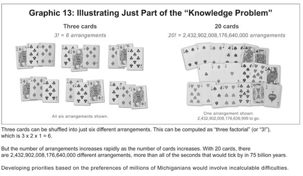
Whatever the effects of political incentives and rent-seeking in MEGA’s economic development efforts, MEGA decisions no doubt usually involve good faith efforts and research by MEGA officials and the business recipients of the MEGA grants. Nevertheless, even this is not likely to advance MEGA’s goal of accelerating job growth above what would have been generated by the market alone. We say this because MEGA officials face an inherent "knowledge problem" that is widely recognized in the economic literature: They cannot reliably determine which corporations will bring the most benefit to the state.
True, most people think of this as a problem that can be solved with good financial research and foresight. But in the book "The Fatal Conceit: The Errors of Socialism," Nobel Memorial Prize-winner F. A. von Hayek explains that "the curious task of economics is to demonstrate to men how much they really know about what they imagine they can design."[163]
He then illustrates the limits on the transmission of information and knowledge that can be accumulated by any small group of planners. Hayek recognized that knowledge is highly diffused and contained in the minds of millions of economic actors who are working to maximize their own self-interest.
The market is the only known method of providing information enabling individuals to judge comparative advantages of different uses of resources of which they have immediate knowledge and through whose use, whether they so intend or not, they serve the needs of distant unknown individuals. This dispersed knowledge is essentially (Hayek’s emphasis) dispersed, and cannot possibly be gathered together and conveyed to an authority charged with a task of deliberately creating order.[164]
In other words, regardless of how talented they are, it is impossible for state officials to know how to redistribute resources in such a way that would make society better off than if they had not intervened. At best, they can hope to get lucky.
To see just how lucky they would need to be, consider the following illustration, devised by the respected Stanford University economist Paul Romer, which helps explain the difficulty in commanding and using information.
There are only six ways to arrange three items (see Graphic 13 above). You can calculate this by using a simple "factorial," where "three factorial" (or "3!"), simply means 3 x 2 x 1, or 6.
But increasing the number of the cards increases the number of potential arrangements at a dramatic rate. With just 20 items, the number of arrangements rockets to 2,432,902,008,176,640,000 — over 2 quintillion, and more than all of the seconds that would tick by in 75 billion years (2,365,200,000,000,000,000).
Now extend that concept to a full deck of 52 playing cards. It is conceivable that some theoretically possible arrangements of a card deck have never actually occurred in any card deck in all of human history.
Yet when economic development officials survey the state economy and try to add more jobs to the state employment rolls than would otherwise exist, they are dealing with potentially millions of items to prioritize, including the varied preferences and plans of the state’s business firms and consumers. Moreover, as Hayek noted, this knowledge is essentially dispersed in people’s minds; it cannot be gathered in the first place.
Track Record of the Private Sector
Thus, even the highest paid and most experienced Wall Street investment experts with scores of analysts at their disposal have trouble picking winners and losers in the marketplace. Ben Warwick, in his book "Searching for Alpha: The Quest for Exceptional Investment Performance," observes that between 1995 and 2000, "Of the 45 largest stock funds, only one has beaten the Standard and Poor’s 500 index . . . and that fund outperformed by a scant 0.60 percent per year."[165]
This is not an uncommon finding. Despite every conceivable advantage in divining which companies are good investments and which are not, and despite enormous economic incentives to succeed, even professional money managers rarely outperform the marketplace as a whole.
In 2002, then-MEDC CEO Doug Rothwell told the managing editor of The Observer Newspapers, "Our philosophy is to support winners, the companies that have a good business model."[166] It certainly sounds like a good strategy, but it’s the strategy employed by most professional investors, and they don’t usually beat the marketplace.
MEGA faces the same "knowledge problem" that plagues central planners in other governments and that makes it hard for private investors to outperform the Standard & Poors Index. They cannot somehow survey the marketplace and a sea of human interaction in all its detail, and then improve it through some state effort, such as targeting tax relief to corporations. It requires knowledge that can never be gathered, assembled and organized. Only millions of individuals acting freely can coordinate the many pieces of local knowledge into a system that is reasonably efficient at improving human wealth.
A Review of the Findings
This study has surveyed MEGA’s evolution during the past 10 years and detailed its track record. As we have seen, MEGA’s original job projections have materialized only in relatively few instances. Even companies that have successfully claimed tax credits under the MEGA program usually fail to create the number of jobs that were advertised in the time frame expected.
Moreover, our detailed econometric analysis of county per-capita personal income, employment and unemployment rate shows that MEGA has had no significant state- or county-level economic impact; indeed, the only measurable impact was often modestly (though not significantly) negative. Our conclusion that MEGA credits did create a temporary shift in employment towards construction jobs is balanced by the findings that MEGA credits had no lasting effect on construction employment and produced no net gain in overall employment. These econometric results are consistent with those of a variety of academic studies of economic development programs like MEGA.
In exploring why MEGA has apparently failed to generate new economic gains, we reviewed a number of possible reasons. First, we examined the uncertain assumptions involved in REMI modeling and the challenges MEGA officials face in determining which firms should receive MEGA credits. Second, we noted that the current economic literature includes at least two broad hypotheses that suggest there are inherent shortcomings of government economic development programs: first, because political and business incentives will tend to overrule good policy; and second, because market economies are too complex for reliable choices about which firms will prove successful.
Our findings thus lead to the question, Should MEGA be abolished, or should it be reformed? Many people will settle this question according to their political philosophy, but we believe the evidence permits an answer that is largely independent of political philosophy or political party.
MEGA, for instance, has been run by Republicans until recently, but similar programs have been overseen by Democrats in Michigan and in other states, and these programs have not enjoyed obvious success, either. Further, state officials have made multiple changes to Michigan’s economic development programs through the years, but these changes have not brought obvious improvements in the programs’ economic impact; indeed, the absence of impact is one reason that officials are moved to make changes in the first place. (For a discussion of the evolution of Michigan’s economic development strategies, see "Appendix E: A Brief History of State Economic Development.") Combined with the review of findings detailed above, it appears that the state of Michigan would be better off eliminating MEGA and concentrating on other policies.
We would add that this conclusion about MEGA is bolstered by several noneconomic considerations. These are spelled out below.
Noneconomic Issues
Constitutional Concerns
In September 2004, the United States 6th Circuit Court of Appeals struck down a state of Ohio economic development program on grounds that it was an unconstitutional restraint of interstate commerce. The decision was rendered in the case Charlotte Cuno, et al. v. DaimlerChyrsler Inc., et al. The plaintiffs included two Michigan residents.
At the heart of the court’s ruling was the U.S. Constitution’s "commerce clause," which vests authority over interstate commerce in the U.S. Congress, not state governments. Ohio had infringed on this congressional power, according to the court, because the state’s economic development program restrained interstate commerce by providing valuable state investment tax credits to corporations that invested in Ohio rather than elsewhere.
This case is widely considered to be a "true test case" of state incentive programs, since the legal challenge was brought primarily against the program’s constitutionality, rather than the particulars of specific decisions made by the program’s officials. Not surprisingly, the state of Ohio appealed the Cuno ruling, which had been made by a three-judge panel, and sought an opinion from the full 12-judge court.
This motion was denied in January 2005. Ohio probably will appeal to the U.S. Supreme Court (the state must decide by mid-April 2005 whether to do so). If the Supreme Court hears the case and upholds the circuit court’s decision, programs like MEGA could all but vanish, since the Ohio program is similar in form to MEGA. As Professor Peter Enrich, one of the Ohio plaintiffs’ attorneys, observes, the MEGA program "is subject to very substantial doubt at this point."[167]
Even if the Supreme Court chooses not to review the case, MEGA tax credit program could be challenged directly by litigants citing the Cuno decision, since Michigan lies in the U.S. 6th Circuit. State officials may soon be forced to evaluate the utility of fighting such a challenge in court, rather than ending the program themselves.
The argument made by the judges in Cuno appears sound. At the margin, the incentives in an economic development program might affect location decisions — they certainly attempt to — and thereby distort interstate investment and trade patterns. Deciding that a firm that locates in Michigan will receive special tax treatment is not significantly different from deciding that the same firm will face a tariff if it locates in Ohio and still tries to do business in Michigan. Such tariffs would clearly be an unconstitutional restraint on interstate trade, so it is difficult to see how a MEGA program passes constitutional muster.
True, some might argue that by the logic above, a "tariff-like barrier" would exist even if Michigan’s tax rates are simply lower across-the-board than those in Ohio. But in a legal sense, the two situations are different. If Michigan lowered its tax rates generally, it would undoubtedly provide an economic incentive for businesses to locate here, but it would in no way discriminate against out-of-state businesses within its own tax code. (Indeed, out-of-state businesses would remain free to locate in states with even lower tax burdens than Michigan’s). The MEGA program, in contrast, distorts Michigan’s tax code in favor of certain in-state firms — and always against out-of-state firms.[168] This attempt to alter the flow of interstate investment violates the purpose of the constitutional bias toward free trade.
Fairness
MEGA’s questionable economic impact and uncertain constitutional status are not the only concerns. A final issue is fairness.
Fairness, admittedly, is not a technical term, and state officials would naturally dispute any suggestion that MEGA’s programs are unfair. Still, given that MEGA does not appear to be meeting its professed goals, the question of its strengths and weaknesses on other measures becomes a legitimate issue in deciding what should be done with the program.
It is unlikely that MEGA comports with the general concept of fairness as it’s understood by most Michigan citizens. When state officials pick "winners" among corporations and other enterprises by offering targeted tax relief, they are implicitly picking "losers," as well — i.e., firms that must pay taxes to support the MEDC, but do not receive MEGA tax credits and must nevertheless compete against firms whose balance sheets are bolstered by such credits.
Consider the situation of the competitors of Lacks Industries Inc. of Grand Rapids. In 1996, Lacks was offered $8.6 million in targeted incentives in the form of MEGA tax credits and other assistance.
As of 1999, for instance, there were 1,395 companies in the state with whom Lacks shared a "Standard Industrial Classification" code, which classifies businesses by industry and economic activity. Businesses within the same SIC code are potential rivals because they often produce similar products or services.[169]
Only six of the 1,395 Michigan companies in Lacks’ SIC code had accepted MEGA deals. Thus, as many as 1,389 Michigan businesses were forced to compete with Lacks without also receiving tax relief from the MEGA program.[170]
The competition between these firms can be intense — as, indeed, Lacks’ 1996 MEGA application shows. The form lists reasons why information about the company should be exempt from public disclosure. Lacks requested this exemption for certain information on grounds that the data would give an "unfair advantage to our competitors."[171]
If it is "unfair" for a firm’s competitors to have information about the firm when the firm doesn’t have the same information about them, it seems at least as unfair for a firm’s competitors to receive tax breaks when the firm doesn’t receive the same tax breaks itself. And since most firms that receive the state’s MEGA grants have rivals not just outside Michigan, but inside Michigan, as well, the state’s sponsorship of MEGA is arguably unfair to many of the state’s own businesses.
Concerns About "Unilateral Disarmament"
As mentioned earlier, a frequent response to public questions about the value of a program like MEGA is to claim that whatever its flaws, ending it would be tantamount to "unilateral disarmament." That is, if other states operate business tax incentive programs, Michigan must do the same, lest it lose economic battles with other states.
But the case is not so clear cut. As Peter Fisher noted when asked by The Detroit News about ending MEGA, "Of course you can unilaterally disarm when you’re talking about an incentive — like the MEGA tax credit — that isn’t very effective anyway."[172]
Thus, ending MEGA and adopting a more effective policy is not unilateral disarmament; it is true armament. Ending MEGA could allow state officials to focus more clearly on broad-based reforms that have a better track record.
After all, every MEGA award is an implicit admission by the state that for that particular firm, it costs too much to do business in Michigan. If this fact is true for a particular business, it is probably true for many of its competitors.
There are 105,000[173] Michigan businesses with Single Business Tax liability. Through December 2004, fewer than 230 of them have enjoyed tax relief through this program. It would not strain economic theory to suggest that these 105,000 businesses would have created as many — if not more — jobs as the MEGA program’s 230 deals if state officials had just cut the Single Business Tax for all of them, instead of targeting tax relief to a handful of enterprises.
Ultimately, the concern over "unilateral disarmament" may become moot. Given the constitutional problems with economic development programs like MEGA, all states may be forced to renounce them. If universal disarmament is coming, Michigan might receive a "peace dividend" by becoming the first to set out on a new path.
Alternative Measures
States do have alternatives to conventional economic development programs. The economic research literature suggests there are other government policies that are more likely to improve a state’s economic growth.
One area of government policy that could produce economic benefits is tax reform, such as lower tax rates, more equitable tax treatment or simplification of the tax code. Michael Wasylenko, for one, has noted the potential problems caused by a policy focus on targeted (or "ad hoc") tax incentive programs, rather than systemic tax reform:
Most important, ad hoc tax reforms should not be used as a back-door remedy to systematic deficiencies in a tax or fiscal system or in the name of improving the business climate. A band-aid approach to tax reform creates more inequities and inefficiencies than it resolves. When the business climate of a state becomes so problematic that tax laws need to be changed routinely to attract businesses, the practice may be a symptom of problems with the tax system itself and a signal that systematic tax reform might be a more useful approach. In effect, tax reform treats existing and new firms equally, and responsible reform will also systematically account for any tax revenue lost due to reform. It is probably the case that sound tax and fiscal policy obviates many of the tax perks that businesses seek.[174]
Lower tax rates in particular could make Michigan’s business climate more competitive. Michigan’s state and local tax burden as a percentage of personal income exceeds the national average, and its corporate tax burden has been called the worst in the nation by the Tax Foundation of Washington, D.C.[175] And lowering taxes might well affect more than business location decisions. For example, economists Robert Genetski and John Skorburg found that an increase in a state’s tax "effort" — a sophisticated measure of tax burden — led to a corresponding decrease in a state’s personal income growth compared to the national average.[176]
There are also signs that the state’s regulatory system is beginning to stifle growth, particularly in areas of telecommunications and environmental regulation.[177] And insofar as government services are a key amenity, Michigan’s public education system continues to generate escalating costs with no corresponding increase in educational quality.[178]
MEGA analyses also frequently cite Michigan’s above-average labor costs. In one such analysis, MEGA officials note that stating that a portion of a company’s "cost differential is attributable to wage rates in (another state) averaging 7 percent lower than in Michigan for the same job classifications."[179] Lower labor costs could take the form of a right-to-work law, which would allow workers to be employed at a unionized firm without joining the union or paying dues to it if they chose not to. One 2002 study found that, from 1970 through 2000, manufacturing employment in right-to-work states has grown at an annual average of 1.7 percent faster than non right-to-work states during the same period.[180]
As we noted above, we are skeptical that reforming MEGA will significantly improve the program’s economic impact. The problems we listed earlier under "MEGA: Explanations" seem likely to undermine attempts to correct the program’s current shortcomings. Our first proposal for reform therefore remains what we suggested above: ending MEGA and pursuing basic reforms to the general policies that shape Michigan’s economic environment.
If policy-makers are unwilling to end the program, we can offer other recommendations for reform that may improve the program’s performance in some ways, though the improvements are not likely to create a meaningful increase the program’s overall economic impact.
Audit MEGA
As we noted earlier, past audits of the state’s economic development programs by Michigan’s Office of the State Auditor General have revealed shortcomings in the programs’ claims of success. In one instance, an audit uncovered that in a report to the Legislature, the Michigan Strategic Fund overstated job claims for two programs by using "company projections rather than actual jobs created."[181] In another instance, the agency failed to investigate closely the jobs creation numbers submitted to it by business grantees.[182]
The state could consider conducting regular, expanded audits of MEGA’s direct job counts. Such oversight might not only clarify the success and failure the authority has achieved, but could encourage more efficient accounting procedures at the authority.
The auditor general’s office could also be encouraged specifically to review applications by MEGA candidates that were rejected. A review of these applications might help determine how many MEGA applicants chose to move to, or expand in, Michigan despite being rejected for MEGA incentives. The results of such a review could help clarify the extent to which MEGA agreements are indeed ensuring that the tax credit is necessary to a firm’s decision to locate in Michigan. The review could also lead to improved procedures for determining which companies should receive the credits.[183]
Count Direct Jobs Only
As we noted earlier, we faced a number of difficulties in determining the basis for the indirect job claims made by MEGA officials (see also "Appendix B: Information Requests to MEDC"). These difficulties suggest how much harder it is to assess the program’s impact when the creation or retention of "indirect jobs" is held to be an important measure of MEGA’s success.
Even if the numbers were transparent and immediately available, they would still be based on assumptions that can prove faulty in retrospect (for instance, see "Failed Employment and Wage Assumptions" in "Technical Considerations in the Modeling Used by MEGA"). Indeed, professional economists of goodwill can quickly disagree over computations of indirect job effects. And ultimately, indirect jobs, unlike direct jobs, are inherently difficult to identify and count, making it harder to challenge nonprofessional estimates of dubious quality (see the discussion of MEGA’s claim of creating 28,812 total jobs in "MEGA Job and Project Performance," under "MEGA's Track Record").
It would probably facilitate public review and understanding of the program if indirect job benefits were no longer reported and cited by MEGA officials. "Spin-off" considerations could still be part of the evaluation process for a particular project, so that a project that promises greater spin-off benefits is more likely to be chosen, but MEGA would no longer make a formal or informal practice of tallying the indirect jobs its past and future projects could claim. Removing MEGA officials’ focus on indirect job counts might free the authority to more carefully document its direct job creation — the issue we addressed in "Audit MEGA," immediately above.
Develop Transparent and Timely Reports
The status of each MEGA project could be posted and updated live on the Web each month to show the following:
the state and local incentives offered in each MEGA package;
the state and local incentives claimed in each MEGA package;
the cost of these incentives so far and in the current year;
the current direct job figures;
what the direct job figures were originally projected to be at present;
what the direct job figures were initially projected to be at the end of the tax abatement period;
what the direct job figures are currently projected to be at the end of the tax abatement period;
a brief and simple assessment of the project’s status based on these figures, such as "currently below targets, but projected to reach them by 2007," or "currently meeting targets but unlikely to maintain them in 2006";
an annual summary of MEGA’s success rate in meeting its targets based on the data above.
Ultimately, MEGA cannot be effective if its program reports are not clear, analytical and open to public scrutiny. Quality improvements at MEGA will be much easier to achieve if a thorough and accessible track record is available to MEGA officials and to the elected officials who evaluate the program’s effectiveness.
Commission an Independent Econometric Review
An independent researcher could be engaged to maintain a peer-reviewed and publicly transparent econometric model that annually reassessed MEGA’s impact. The model we employed in this study[184] is crafted to detect past impact, rather than predict future performance. Regular updates of the findings would therefore be appropriate if MEGA continues.
A number of qualified university academics could undertake such research. The University of Michigan’s world-renowned Office of Tax Policy Research would be eminently qualified to perform such an evaluation. If it were deemed more appropriate to find researchers outside the University of Michigan, Syracuse University, Harvard University and the University of Tennessee all operate top-notch programs with which the state might contract for an econometric evaluation of the MEGA program.
1 Kenneth P. Thomas, Competing for Capital: Europe and North American in a Global Era (Washington, D.C.: Georgetown University Press, 2000).
2 Alan Peters and Peter Fisher, "The Failures of Economic Development Incentives," Journal of American Planning Association. 70:1 (2004): 28.
3 All MEGA Projects, State of Michigan, Michigan Economic Development Corporation e-mail to Michael D. LaFaive, December 21, 2004.
4 John Engler, Journal of the Senate, State of Michigan, (1984), 2483.
5 Chris Christoff, "Engler pushes for states to end fights over business," Detroit (MI) Free Press, sec. E. Aug. 5, 1992.
6 Maria Tyszkiewicz, "The Economic Development Programs of the Michigan Jobs Commission," State of Michigan, Senate Fiscal Agency (December 1998), https://www.senate.michigan.gov
7 Michigan Economic Growth Authority Act (April 18, 1995), Michigan Compiled Laws Annotated, sections 207.1 (West Group) 1998.
8 Ibid.
9 Martin Wing, Robert Fish, and Joseph Overton, MEGA Industrial Policy: An Analysis of the Proposed Michigan Economic Growth Authority, Midland, Mich.: Mackinac Center for Public Policy, March 1995.
10 Donald Jakeway, This Week @ MEDC, e-mail to unknown list, including Michael D. LaFaive, State of Michigan, Michigan Economic Development Corporation, April 27, 2004.
11 Public Act 144 of 2000, State of Michigan (michiganlegislature.org), 90th Legislature, June 6, 2000: 4.
12 House Legislative Analysis Section, "Brownfield Redevelopment," Lansing, Mich: State of Michigan. 2000: 2.
13 Ibid., Public Act 144 of 2000, State of Michigan (michiganlegislature.org): 5.
14 "Bill Analysis (Public Act 428 of 2000 and Public Act 429 of 2000)," Lansing, Mich: State of Michigan, Senate Fiscal Agency, January 16, 2001: 1.
15 Maria Tyszkiewicz and Jay Wortley, "Bill Analysis," Lansing, Mich: State of Michigan, Senate Fiscal Agency, December 16, 2003: 3. The original quote referred to 2,000 jobs, but the bill was evidently altered afterwards.
16 Public Act 248 of 2003, State of Michigan (michiganlegislature.org), 92nd Legislature, December 2003: 1-6.
17 Ibid.
18 Public Act 81 of 2004, State of Michigan (michiganlegislature.org), 92nd Legislature, April 2004: 5.
19 Public Act 398 of 2004, State of Michigan (michiganlegislature.org), 92nd Legislature, October 15, 2004: 5.
20 Ibid., All MEGA Projects; and MEGA Credits, State of Michigan, Michigan Economic Development Corporation e-mail to Michael D. LaFaive, December 7, 2004.
21 Ibid., All MEGA Projects.
22 It was not always easy to determine when a MEGA deal was being provided to a parent corporation, as opposed to a listed subsidiary or supplier of that corporation. Furthermore, deals listed as separate MEGA initiatives may have required the approval of a larger corporation in order to be sanctioned. For instance, if three General Motors suppliers received MEGA deals contingent on GM’s decision to refurbish a plant, the MEGA packages could be counted as three deals or as one, depending on the method employed. Both we and the MEDC count these as three deals.
23 Ibid., All MEGA Projects.
24 Ibid., Michigan Economic Growth Authority Act.
25 Ibid., All MEGA Projects.
26 Ibid.
27 Authors’ calculations based on the following: ibid., All MEGA Projects; Briefing Memos, State of Michigan, Michigan Jobs Commission and Michigan Economic Development Corporation, sent by Michigan Jobs Commission and Michigan Economic Development Corporation to Michael D. LaFaive under the Michigan Freedom of Information Act on multiple dates between 1995 and December 2004; Michigan Economic Growth Authority Annual Report, Lansing, Mich: State of Michigan, Michigan Economic Development Corporation, years 1995 through 2004.
28 Some MEDC documents detail the value of so-called "Renaissance Zone" tax relief, while others are less specific.
29 John Truscott, "State Incentive Package Approved to Attract Further GM Investments in Michigan," State of Michigan: Executive Office, June 13, 2000: 2.
30 Ibid., All MEGA Projects.
31 According to an October 14, 2003 MEDC Briefing Memo, "General Motors will make the ultimate location decision on this project; however, without the MEGA tax credits the suppliers will not be able to provide General Motors with the required cost savings necessary to make this project viable."
32 Some of the authors’ unsuccessful efforts to obtain clarifications about MEDC data are described in "Appendix C: Determining MEGA’s Job Counts." An earlier version of the material in this appendix also appears at www.mackinac.org/6992.
33 On March 29, 2005, MEDC spokesman Paul Krepps answered an important question about MEGA’s methodology for tallying credits and indirect job counts. Other questions have been submitted to the MEDC starting in January 1, 2005 or earlier, and although the MEDC has agreed to answer these, the answers will not arrive before publication of this study.
34 Donald Jakeway, "Gripes against MEDC flawed," Business Direct Weekly, p. 6, November 4, 2004.
35 David Hollister, "MEGA is vital tool for creating jobs, growth," The Detroit (MI) News, sec. A, September 19, 2003.
36 Authors’ calculations based on the following: ibid., All MEGA Projects; ibid., MEGA Credits; and Economic Effects, Lansing, Mich: State of Michigan, Michigan Economic Development Corporation, years 1995 through 2004.
37 To date, MEDC documents indicate that only 77 companies have met the bare minimum requirement of creating 75 (sometimes 150) qualified new jobs (usually) within one year of beginning work at a new facility.
38 Ibid., MEGA Credits.
39 "Labor Market Information Quick Stats," State of Michigan, Michigan Department of Labor and Economic Growth, December 2004, www.michlmi.org.
40 Mark Hornbeck, "Tax breaks shortchange state: $1.4B business program gets minimal payback in jobs," The Detroit (MI) News, sec. A, September 2, 2003.
41 Ibid., Don Jakeway, Business Direct Weekly.
42 Ibid., MEGA Credits.
43 See "Appendix C: Determining MEGA’s Job Counts" for a discussion of our methodology in computing direct job counts. (An earlier version of this appendix appears at www.mackinac.org/6992. For the document indicating that the larger figure was due to indirect job counts, see particularly the penultimate hyperlink in that piece, which can be reached directly at www.mackinac.org/archives/2005/medc102604.pdf.)
44 MEDC spokesman Paul Krepps, e-mail message to author Michael D. LaFaive, March 29, 2005.
45 We discuss REMI’s use in MEGA projections in "Technical Considerations in the Modeling Used by MEGA."
46 We calculated that 56 projects were involved along the lines described earlier in "MEGA Job and Project Performance" in "MEGA's Track Record." Our methodology for this calculation is described in greater detail in "Appendix C: Determining MEGA’s Job Counts."
47 In the March 29, 2005 e-mail message cited in endnote 44, MEDC spokesman Paul Krepps indicates that the ratio is based on 56,103 direct jobs and 62,301 indirect jobs. These figures are a total of all projected past and future direct and indirect jobs arising from MEGA projects. This use of jobs that are being projected for the future is the basis for the some of our criticism of the MEDC’s approach, as explained in the text.
48 Ibid., Don Jakeway, Business Direct Weekly. See specifically the statement "[O]f the MEGA projects that have collected SBT credits for their projects to date, 28,812 total jobs have been created. ..."
49 See, for instance, Executive Budget Appendix on Tax Credits, Deductions, and Exemptions, Fiscal Year 2005, Lansing, Mich.: State of Michigan, Michigan Department of Treasury: 36.
50 Ibid., Don Jakeway, Business Direct Weekly.
51 Ibid., Executive Budget Appendix on Tax Credits, Deductions, and Exemptions, Fiscal Year 2005: 36.
52 Executive Budget Appendix on Tax Credits, Deductions, and Exemptions, Fiscal Year 2004, Lansing, Mich.: State of Michigan, Michigan Department of Treasury: 37.
53 John Truscott, "Southeast Michigan Jobs Bonanza: 2,891 New Jobs Coming to Michigan: Delphi Automotive Systems Builds in Troy," State of Michigan: Executive Office, June 13, 2000. The news release is referring to three companies that received MEGA agreements: Delphi Automotive Systems, LDM Technologies Inc. and Altair Engineering Inc.
54 John Truscott, "1,160 New Jobs for Michigan! 12,000 MEGA Jobs are Helping Michigan Drive America’s Renaissance," State of Michigan: Executive Office, March 12, 1996. The news release is referring to jobs at three companies: Case System Inc., National TechTeam Inc. and Shape Corp.
55 John Truscott, "Greater Detroit Area Beats out Toledo for Webvan Group, Inc. Facility: 1,198 New Jobs for State," Michigan Government News, December 21, 1999.
56 Tim Venable, "Consummate consumer service: Site Selection’s 1999 top 10 development groups," Site Selection: May 2000: 8.
57 Case Systems had an early, small success, but subsequent job cuts have led to a loss of access to credits.
58 Webvan Group Inc. stock value plummeted from more than $18 a share to just 0.47 cents in those 12 months, and it ultimately went lower.
59 Ibid., MEGA Credits.
60 Daniel Hauck, "Delphi hits the bottom of S&P 500 companies," Detroit (MI) Free Press, sec. C, March 30, 2005.
61 Authors’ calculations based on the following: Briefing Memo: Kmart Corp., State of Michigan, Michigan Jobs Commission, May 1998; Briefing Memo: Kmart Corp., State of Michigan, Michigan Economic Development Corporation, August 2000; ibid., All MEGA Projects, Michigan Economic Growth Authority: 1998 Annual Report, Lansing, Mich: State of Michigan, Michigan Jobs Commission; Michigan Economic Growth Authority: 2000 Annual Report, Lansing, Mich: State of Michigan, Michigan Economic Development Corporation.
62 Ibid.
63 United States Bankruptcy Court, Northern District of Illinois Eastern Division, Case No. 02 B 02462 through 02 B 2494 and Kmart Corp., "Shareholders FAQs," www.kmartcorp.com/corp/investor/general/faq.stm.
64 Ibid., see note 61.
65 MEGA Tax Credit Agreement: Kmart Corp., Schedule A," State of Michigan, Michigan Jobs Commission, effective June 18, 1998.
66 MEGA Tax Credit Agreement: Kmart Corp., Schedule A," State of Michigan, Michigan Jobs Commission, terms accepted Aug. 31, 2000.
67 Daniel Howes, "State Feels Jilted by Kmart: Merger comes while officials were offering millions in tax breaks to keep Troy headquarters," The Detroit (MI) News, sec. A, November 18, 2004.
68 R.J. King and Tenisha Mercer, "Cities tailor incentives to lure Kmart: Detroit, Pontiac, Troy aim to outshine each other, Atlanta," The Detroit (MI) News, sec. B, October 29, 2004.
69 MEDC Freedom of Information Act Officer Theresa Rashid, letter to Michael D. LaFaive, "The total amount of SBT credits that Kmart has received for the two projects through their 2001 tax year is $6,102,215," January 24, 2003.
70 Briefing Memo: Covisint, LLC, State of Michigan, Michigan Economic Development Corporation, Nov. 13, 2001: 1.
71 Rick Haglund, "It ain’t pretty, but it just may work," Booth Newspapers, September 13, 2000. The Detroit Free Press reported a slightly lower estimate of $240 billion annually in brokered sales: See Jamie Butters and Jeff Bennett, "Business is falling flat for Covisint," Detroit Free (MI) Press, sec. A, December 9, 2002.
72 Ibid., Jamie Butters and Jeff Bennett, Detroit (MI) Free Press.
73 Official Meeting Minutes (November 13, 2001), State of Michigan, Michigan Economic Development Corporation, Nov. 13, 2001: 4.
74 MEGA Tax Credit Agreement: Covisint, LLC, Schedule A," State of Michigan, Michigan Jobs Commission, terms of the agreement accepted January 21, 2002.
75 Ibid., Jamie Butters and Jeff Bennett, Detroit (MI) Free Press: p. 8A.
76 Ellen Messmer, "Compuware to acquire Covisint B2B exchange," ComputerWorld, February 5, 2004 (available on the Web at www.computerworld.com/news/special/pages/story/ 0,5364,1865-89896,00.html).
77 Matthew Schifrin, "B2B’s Back," Forbes.com, available on the Web at www.communicate.com/news_display.php?newsID=100.
78 Compuware Corp. staff member Paulette Kane, telephone interview with Michael D. LaFaive, January 25, 2005.
79 Other cases of failed MEGA investment can be found in past publications by the Mackinac Center for Public Policy; see the Center’s Web site at www.mackinac.org/depts/ecodevo/. The Mackinac Center’s first study on the subject of government economic development programs in Michigan, published in 1989, focused on regional economic development and warned that ad hoc policies that relied on property tax abatements and other local incentives were not likely improve longterm employment opportunities and economic growth (see Greg Kaza and Gary Wolfram, Regional Economic Development: Downriver As A Case Study (Midland, Mich.: Mackinac Center for Public Policy), available on the Web at www.mackinac.org/274.) Since that time, Center scholars have written three studies (including this one), 12 Viewpoint Commentaries, dozens of Web-only essays, several exclusive newspaper Op-Eds and scores of speeches on a variety of government economic development initiatives.
80 Michael D. LaFaive, MEGA: Real Jobs or Smoke and Mirrors (Midland, Mich.: Mackinac Center for Public Policy, December 1999, available on the Web at www.mackinac.org/2592).
81 In 2003, Robert Bosch reduced its staffing in Kentwood, Mich., by 1,200 employees, and the firm is expected to lay off another 500 workers in St. Joseph throughout 2005.
82 Current Employment Statistics (Detailed State and Metro Area Statistics customized table), U.S. Department of Labor, Bureau of Labor Statistics, available on the Web at www.bls.gov/sae/home.htm, accessed on January 30, 2005.
83 Current Employment Statistics (Detailed State and Metro Area Statistics customized table), U.S. Department of Labor, Bureau of Labor Statistics, available on the Web at www.bls.gov/sae/home.htm, accessed on March 28, 2005.
84 Just The Facts: Key Economic and Social Indicators for New York State: Total Private-Sector Employment, Public Policy Institute of New York State, available on the Web at www.ppinys.org/reports/jtf2004/privsectemploy.htm, accessed in December 2004.
85 Authors’ calculations based on the following: Regional Economic Accounts ( Gross State Product customizable table), U.S. Department of Commerce, Bureau of Economic Analysis, available on the Web at www.bea.gov/bea/regional/gsp/; Regional Economic Accounts ( State and Local Personal Income customizable table), accessible on the Web at www.bea.gov/bea/regional/spi/.
86 Regional Economic Accounts (State and Local Personal Income customizable table), U.S. Department of Commerce, Bureau of Economic Analysis, available on the Web at www.bea.gov/bea/regional/spi/.
87 "Michigan Has No. 1 Jobless Rate," Michigan Information and Research Service, January 25, 2004, available to subscribers on the Web at www.mirsnews.com/capsule.php?gid=166#2537.
88 State Employment Statistics – December 2004, Joint Economic Committee of the United States Congress, available on the Web at www.jec.senate.gov.
89 Jennifer Bonham, "West And Southeast Gain In Appeal, North Sees More Leaving According To Latest United Van Lines Migration Study," (Fenton, Missouri: United Van Lines, January 6, 2005, available on the Web at www.unitedvanlines.com/media/press/2005.htm.)
90 Ibid., MEDC Freedom of Information Act Officer Theresa Rashid, letter to Michael D. LaFaive.
91 Michael Wasylenko, "Taxation and Economic Development: The State of the Economic Literature," New England Economic Review, March/April 1997: 37-52.
92 Ibid.
93 Todd Gabe and David S. Kraybill, "The Effect of State Economic Development Incentives on Employment Growth of Establishments," Journal of Regional Science, 42:4 (2002): 703.
94 Terry F. Buss, "The Effect of State Tax Incentives on Economic Growth and Firm Location Decisions: An Overview of the Literature," Economic Development Quarterly, 15:1 (2001): 99.
95 Ibid., Alan Peters and Peter Fisher, Journal of the American Planning Association: 27.
96 Ibid.: 32
97 Ibid.: 35.
98 Timothy J. Bartik, "Evaluating the Impacts of Local Economic Development Policies On Local Economic Outcomes: What Has Been Done and What is Doable?" (working paper, Upjohn Institute Staff, Upjohn Institute, Kalamazoo, Mich., Working Paper No. 03-89, 2000.)
99 For a detailed explanation of measurement errors in these types of studies, see W. Robert Reed and Cynthia Rogers, "Measurement Error and Endogeneity in Studies of State Tax Policy and Economic Growth," (working paper, University of Oklahoma, Department of Economics, Norman, Oklahoma, 2000).
100 Kelly Edmiston, "The Net Effects of Large Plant Locations and Expansions on County Employment," Journal of Regional Science, 44:2: 289-319.
101 William F. Fox and Matthew Murray, "Do Economic Effects Justify the Use of Fiscal Incentives?" International Regional Review, 24:1: 103-133.
102 Michael J. Hicks, "The Regional Impact of Wal-Mart Entrance: A Panel Study of the Retail Trade Sector in West Virginia," Review of Regional Studies, 31:3: 305-313; and Michael J. Hicks, "A Quasi-Experimental Test of Large Retail Stores Impacts on Regional Labor Markets: The Case of Cabela’s Retail Outlets," (working paper).
103 Manufacturing firms and warehousing were eligible for the credits. Construction firms do not receive the credits directly, but construction activity will have accompanied many of the projects.
104 As a technical aside, the possibility exists that the MEGA credits were targeted to poorer places (despite that not being a formal criterion). The instrumental variable approach was specifically designed to account for this possibility.
105 The reverse could be true. We could have detected positive gains for MEGA counties that did not produce statewide benefits, most likely because the gains to MEGA counties came from reallocated economic activities from non-MEGA counties, thereby rendering the net effect zero.
106 We can conclude that the activity is a shift, since there is no corresponding population growth.
107 The $123,000 is only the value of the tax credit. This does not include the value of other incentives, or the fully allocated cost of MEGA staff and of the business recipients.
108 MEDC Freedom of Information Act Coordinator Sara Galluch, letter to Michael D. LaFaive, January 19, 2005.
109 In fact, a REMI expert with whom we conferred told us, "The guys at U of M are very good with the model."
110 George Fulton, Donald Grimes, Peter Nicolas, "The Economic Effects on Michigan of the Solvay Plant Location Decision," Economic Effects, Lansing, Mich: State of Michigan, Michigan Economic Development Corporation, April 20, 1995: 2.
111 In fact, the cost would be even higher than just simply the amount of the MEGA package that was unnecessary to keep or bring the company to Michigan. Officials at REMI, the Amherst, Mass., business that programs and sells the software model, encourage their clients to "identify even a minimal assumption of the opportunity costs on those government funds (NPV of T-bill rate) and include [it] in the model." At the same time, this cost would have a minimal impact on estimates — if any — even if it were factored in.
112 Authors’ calculations based on the following: ibid., All MEGA Projects; ibid., MEGA Credits; and ibid., Economic Effects, years 1995 through 2004.
113 There is another ramification of the model’s inability to distinguish between different regions in the state: It cannot distinguish MEGA projects close to a Michigan border from those far from it. It thus will have difficulty accounting for spin-off business activity that is sent to out-of-state businesses, rather than to in-state businesses from a MEGA project. A business that receives a MEGA grant in Detroit or Coldwater, for example, may spend a significant share of the money resulting from its MEGA package to buy items from Ontario or Indiana suppliers, thereby creating new jobs and income outside, rather than inside, the state — something the REMI model would have difficulty recognizing. Such a dynamic would lead the REMI model to overstate the economic impact of a MEGA grant on the state’s economy.
Of course, it is also possible that cross-border trade could bring new spending from out of state to Michigan. If it did so at a significant rate, it is possible that the REMI model would understate impact of a MEGA grant. Thus, while it is unclear whether this cross-border impact on the whole leads to overstatements or understatements of the economic impact, it is probably one meaningful source of potential error in the REMI modeling.
Cross-border traffic is not a trivial concern. Michigan shares borders with Ohio, Indiana, Ontario and even Wisconsin, and 62 of MEGA’s projects are near one of these borders. Some firms receiving a MEGA package may have branches in one of these four cross-border areas and do significant trade with them. Attempts to crowbar a correction factor into the single-state REMI model to account for this problem would almost certainly cause more problems with the model than the cross-border factors the correction was trying to address in the first place.
114 Timothy Bartik, Peter Eisinger and George Erickcek, "Economic Development Policy in Michigan," Michigan at the Millennium, Lansing, Mich.: Michigan State University Press, 2003: 293.
115 Ibid.
116 Michael D. LaFaive, MEGA Program Shifts Jobs to Where They Are Needed Least, (Midland, Mich.: Mackinac Center for Public Policy, April 7, 1999, available on the Web at www.mackinac.org/3190).
117 Charles Crumm, "Affluent Oakland, Where do we rank?" The Daily Oakland (MI) Press, April 23, 2004, accessed on the Web on April 7, 2005 at www.theoaklandpress.com/stories/042304/loc_20040423073.shtml. This ranking is derived from federal median household income data by Oakland County officials. It reflects a ranking of counties with a population of at least 1 million people. In a ranking of all American counties, Oakland drops to 33rd.
118 Ibid., Michigan Economic Growth Authority Act, Michigan Compiled Laws Annotated.
119 Ibid.
120 Ibid., All MEGA Projects.
121 Michigan Information and Research Service, April 21, 1995: 3 (quoting from The Ann Arbor News)
122 Ibid.
123 Briefing Memo-Compuware Corporation, State of Michigan, Michigan Jobs Commission, September 24, 1996: 2.
124 Daniel Fricker, "Compuware plays it safe," Detroit (MI) Free Press, May 6, 1999, accessed on the Web at www.freep.com/business/qcomp6.htm.
125 Official Meeting Minutes (September 2001), State of Michigan, Michigan Economic Development Corporation, September 2001: 2.
126 For one description of our efforts to obtain this information, see Michael D. LaFaive, Job Search, (Midland, Mich.: Mackinac Center for Public Policy, March 1, 2005, available on the Web at www.mackinac.org/6992). The efforts to obtain this information have been extended. First, author Michael D. LaFaive was told rejected applications weren’t kept; then, he was told that they existed but were spread across state government and might cost as much as $10,000 to locate and copy. In October 2004, he made another request for these applications, which ultimately produced the five applications mentioned in the text.
127 Ibid., Timothy Bartik, et al., "Economic Development Policy in Michigan": 289.
128 Lawrence Reed, Time to End Economic War Between the States, (Midland, Mich.: Mackinac Center for Public Policy, April 4, 1996, available on the Web at www.mackinac.org/718).
129 Ibid.
130 It is true that some surveys have purported to find that tax incentives matter. For instance, Area Development magazine’s 2003 "Corporate Survey" actually ranked incentives as the number one variable in a host of other options based on a survey it had conducted of its readers. The sample in this poll, however, was more likely to be skewed than the two samples of the surveys cited in the main text, since the sample in the Area Development poll was self-selected. Area Development magazine is a professional publication that covers site selection and relocation, and it sends its survey questions to its subscribers. It is not hard to imagine that people who are in the business of providing and receiving business incentives might find incentives to be important in the site location process.
131 Nobel Memorial Prize-winning economist James Buchanan has pioneered a branch of economics known as "public choice" economics, which superimposes the market model of self-interest on government officials.
132 Margaret E. Dewar, "Why State and Local Economic Development Programs Cause So Little Economic Development," Economic Development Quarterly, 12:1 (1998).
133 Ibid.: 68.
134 Ibid.: 87.
135 Matt Resch and Bill Nowling, "Republicans Vow: ‘We Will Fight For Every Michigan Job,’" Michigan Legislature, Office of House Speaker Rick Johnson, October 27, 2004: 1.
136 It is hard not to become cynical when reviewing these documents. State officials and their staffs spend a significant amount of time and taxpayer resources on programs meant to develop the economy, yet the economic value of these programs is not even mentioned in important internal communications. Supporters of the programs sometimes respond that "politicians always engage in politics," but this "realist’s view" actually concedes a decisive point: that the programs are serving political purposes, and that the economic impact is at most an afterthought.
An equally relevant issue is whether in politicians’ attempt to "do something," they are spending money ineffectively and perhaps even hurting job-seekers in the long run. Consider the trade-off involved in passing of the "Jobs II" package. In 2004, Gov. Granholm proposed a cigarette tax hike of 75 cents per pack to help raise revenue and close an expected state budget deficit. The Mackinac Center for Public Policy estimated that the hike would cause a loss of 5,000 jobs in Michigan in the 12 months following the increase. According to the Lansing-based Michigan Information and Research Service, in May 2004, Senate Majority Leader Sikkema offered to trade Gov. Granholm GOP approval of her tax increase for her support of the GOP Jobs I and Jobs II packages advanced in the previous year (see "Sikkema wants Jobs II for Cig Tax," Michigan Information and Research Service, May 27, 2004). It is quite possible, then, that in the passage of the Jobs II program and the cigarette tax, the political price of a program to "create jobs" was a political program that killed jobs.
137 Hemlock Semiconductor Corporation Site Manager Greg Skufca, general memo to employees, November 30, 2004.
138 Ibid., Hemlock Semiconductor Corporation Site Manager Greg Skufca, general memo.
139 Hemlock Semiconductor Site Manager Greg Skufca, telephone interview with Joseph G. Lehman, April 7, 2005.
140 Ibid., Asked about economic development in Michigan, Mr. Skufca stated that high energy and labor costs make Michigan a difficult place to do business.
141 Paul Krepps, "Hemlock Semiconductor to Expand in Saginaw Area, Create Over 120 New Jobs," State of Michigan, Michigan Economic Development Corporation, November 16, 2004.
142 Performance Audit of the Michigan Strategic Fund, Department of Commerce, October 1, 1988 through Oct. 31, 1992, State of Michigan, Office of the Auditor General, July 22, 1993: ii.
143 Ibid., Don Jakeway, Business Direct Weekly.
144 Editorial, "Jobs promise lost," Toledo (OH) Blade, Sept. 20, 2003, accessible on the Web at www.toledoblade.com/apps/pbcs.dll/ artikkel?SearchID=73148341519429&Avis=TO&Dato=20030920&Kategori=OPINIO N02&Lopenr=109200151&Ref=AR.
145 Ibid.
146 Joe Mahr, "Growth agency takes less credit: Analysis redefines, reduces project numbers," Toledo (OH) Blade, June 25, 2004, available on the World Wide Web at www.toledoblade.com/apps/pbcs.dll/ artikkel?SearchID=73197141456084&Avis=TO&Dato=20040625&Kategori=NEWS17 &Lopenr=406250352&Ref=AR.
147 Ibid.
148 Ibid.
149 Ibid.
150 Robert Johnson, "Advocates of Tax Breaks See Software as an Ally," The Wall Street Journal, sec. F, January 22, 1997. Journalists are not the only ones to observe the effect that computer models can have on public acceptance of the claims of government jobs programs. In "The Misuse of Regional Economic Models," a paper by distinguished real estate and finance scholar Edwin Mills of Northwestern University in Chicago, Mills suggests how advocates of various "economic development" programs can use regional economic models to advance their own agendas (see Edwin Mills, "The Misuse of Regional Economic Models," Cato Journal, 13:1, Spring/Summer 1993: 38). The Mills paper analyzed REMI’s use in impact studies particularly for government projects like convention centers and sports stadiums, though it’s clear from his discussion that his observations apply to government development programs more broadly. Mills concludes his paper by offering the "the following conjecture to stimulate thought":
First, government officials like to promote big government. They benefit from large government roles in the economy. Adequate evidence is the observation that state and local governments resist cutting spending and, indeed, frequently raise taxes, in recessions when taxpayers’ ability to pay has decreased. Second, to justify increased spending, government officials must identify some publicly desired goal to be accomplished by government spending. Creation of new jobs is among the best such goals that can be found. Third, they must make it plausible that government can accomplish the goal in a way that the private sector cannot. This is where REMI is so valuable. It is a complex computer model that lay people cannot understand or evaluate, and it has important scientific merits. Thus, the frequent government claim that the best scientific model available shows that x thousand jobs will be created by the project helps to carry the day.
151 Ibid., MEDC Freedom of Information Act Officer Theresa Rashid, letter to Michael D. LaFaive: 10. This figure excludes alleged direct and indirect jobs retained through MEGA programs.
152 Ibid.: 13.
153 Ibid., MEDC Freedom of Information Act Coordinator Sara Galluch, letter to Michael D. LaFaive.
154 Michigan Economic Growth Authority Act (April 18, 1995), Michigan Compiled Laws Annotated, section 207.801 (West Group) 1998: 304.
155 Ibid., MEDC Freedom of Information Act Coordinator Sara Galluch, letter to Michael D. LaFaive.
156 Todd Gabe and David Kraybill, "The Effect of State Economic Development Incentives on Employment Growth of Establishments," Journal of Regional Science, 42:4 (2002): 703.
157 Donald Bartlett and James Steele, "What Corporate Welfare Costs," Time, Nov. 9 1998 (reprint of a special report on corporate welfare; no page number provided).
158 Jean Wylie, Poletown: Community Betrayed, (Champaign, Ill.: University of Illinois Press, 1989), 36.
159 These words were taken from an appeals court decision concerning a dispute between Ypsilanti Township and General Motors regarding tax abatements (see Ypsilanti Township v. General Motors Corp., 201 Mich App 128; 506 NW2d 556 (1993), lv den 443 Mich 882; 509 NW2d 152 (1993) (Michigan Appellate Court, 1993)). The opinion can be found on the Web at www.courtofappeals.mijud.net/Digest/newHTML/ 16124521.htm#TopOfSynopsisMichigan.
160 Harold Brumm, "Rent Seeking and Economic Growth: Evidence from the States," Cato Journal, 19:1 (1999): 7.
161 Ibid.: 15.
162 Ibid.: 7.
163 F. A. Hayek, The Fatal Conceit: The Errors of Socialism, ed. W. W. Bartley III (Chicago: The University of Chicago Press, 1989): 76.
164 Ibid.: 77.
165 Joseph Dancy, "Why do mutual fund managers underperform?," review of Searching for Alpha: The Quest for Exceptional Investment Performance, by Ben Warwick, Financial Sense University, March 25, 2004, www.financialsense.com/fsu/posts/dancy/reviews/032504.html.
166 Hugh Gallagher, "Rothwell injects a welcome shot of optimism on economy," Livonia Observer, sec. A, March 7, 2002.
167 Michael D. LaFaive, United States Circuit Court of Appeals Finds Ohio’s Targeted Investment Tax Credit Unconstitutional, (Midland, Mich.: Mackinac Center for Public Policy, September 2, 2004, available on Web at www.mackinac.org/6802).
168 The authors thank Professor Peter Enrich, the plaintiff’s attorney cited in the text, for his insights on this issue, which formed the basis of the argument we present here.
169 These SIC codes have, at least in the past, been vital to REMI software in estimating the impact of policy changes on employment and other variables of interest.
170 Michael D. LaFaive, Picking Winners and Losers with Tax Credits Is Unnecessary and Unfair (Midland, Mich.: Mackinac Center for Public Policy, July 5, 1999: 2).
171 Ibid.
172 Mark Hornbeck, "Tax breaks shortchange state: $1.4B business program gets minimal payback in jobs," The Detroit (MI) News, sec. A, September 2, 2003.
173 Michigan Department of Treasury staff member Denise Heidt, telephone interview with Michael D. LaFaive, November 3, 2004.
174 Ibid., Michael Wasylenko, New England Economic Review.
175 Tax Foundation, State Business Tax Climate Index, October 14, 2004, www.taxfoundation.org/sbtci.html.
176 Joseph and Diane Bast, ed., "Coming Out of the Ice," Heartland Institute PolicyBot, April 11, 2005, www.heartland.org/pdf/16042.pdf.
177 Diane Katz, A Telecommunications Policy Primer: 20 Comprehensive Answers to 20 Basic Questions (Midland, Mich.: Mackinac Center for Public Policy, August 2004, available on the Web at www.mackinac.org/6750).
178 Andrew Coulson, No Cop Out Left Behind, (Midland, Mich.: Mackinac Center for Public Policy, March 23, 2005, available on the Web at www.mackinac.org/7010; Brian Carpenter, 4M: The Real Structural Problem," www.mackinac.org/6983.
179 Briefing Memo – La-Z-Boy, Inc.," State of Michigan, Michigan Economic Development Corporation, December 21, 1999: 2.
180 William Wilson, The Effect of Right-to-Work Laws on Economic Development (Midland, Mich.: Mackinac Center for Public Policy, June 2002: 2, available on the Web at www.mackinac.org/4290). This is not the only study to find that Right-To-Work states — known as RTW states — enjoy higher employment growth. See, for instance, Thomas Holmes, "The Effect of State Policies on the Location of Industry: Evidence from State Borders," Federal Reserve Bank of Minneapolis, Research Department Staff Report, September 1996: 2. Holmes, an economist at the Federal Reserve Bank of Minneapolis, explains that from 1947 (the year Michigan’s first prominent economic development program was created) to 1996, manufacturing employment in non-RTW states "is virtually the same today as it was in 1947 and 10 percent less than it was in 1963." By contrast, Holmes found that RTW states have seen a 150 percent increase in manufacturing employment.
181 Ibid., Michigan Office of the Auditor General, Performance Audit of the Michigan Strategic Fund, Department of Commerce: October 1, 1988 through October 31, 1992.
182 Performance Audit of Selected Training Related Programs, Michigan Economic Development Corporation, State of Michigan, Office of the Auditor General, August 2003: 11-14.
183 As noted elsewhere (see "A Lack of Data on Rejected Firms" under "The Problem of Ensuring MEGA Credits Are Necessary"), we have attempted to obtain these documents from the MEDC. While the MEDC did supply us with several of the failed applications, it seems likely that there are other applications that our FOIA request did not successfully unearth.
184 For a general discussion of the model, see "Modeling the Economic Impacts of MEGA" under "Econometric Evaluation of MEGA's Effectiveness." For a more detailed description, see "Appendix A: The Model of MEGA’s Economic Impacts."
In order to evaluate the impact of MEGA credits on employment, income and unemployment rates we constructed a time series cross sectional model of Michigan's economy. We obtained data on MEGA credits by county, standard industrial classification, firm, date of approval, project start date and the period over which the credits would be applied. Data on aggregate employment and incomes were collected from the Bureau of Labor Statistics, Regional Economic Information System. These data are readily available from 1969 through 2003. We report the 1990-2003 results as this is the time immediately prior to and during the MEGA credit period.
The model we estimate is of the type commonly employed to evaluate regional policy changes and impacts such as MEGA credits (it is formally known as a "fixed-effects instrumental variable model with spatial and time autocorrelation functions"). This model allows a testing of the magnitude and direction of an impact – here, the MEGA credits – upon aggregate and sectoral employment and incomes. The model accounts for long run trends in the economy, the business cycle, labor force participation rates and the impact of adjoining counties on employment and income in each of Michigan's counties. It takes the general form:
where:
X is aggregate or sectoral employment or income or total unemployment rate;
α, an intercept;
β1, the coefficient for the value of MEGA credits contemporaneously;
The β2 coefficient is for a recession dummy RECC;
β3, the coefficient on the labor force participation rate;
δ1, the coefficient estimate for the spatial autocorrelation variable Xi-s;
δ2, the coefficient for the recursive spatial autocorrelation variable Xi-s,t-n;
φ1 to Xt-n, the autocorrelation component;
γi, the fixed effects intercept;
εt, the error term where we assume εt → iid N(0,σ).
This panel model was estimated using both ordinary least squares and a two stage least squares instrumental variable approach. The instrumental variables included the lagged dependent variables and an instrument representing the date the MEGA project was approved (there is much variation, but a two year lag from the start date of the project is common). This approach exploits the potential endogeneity of entry decisions with the error term. This is almost identical to a technique employed in a similar context by Basker (2005) in his estimate of the impact of Wal-Mart on retail productivity. The use of lagged independent variables as the remaining instruments is a common application in panel models to account for potential endogeneity. This is especially of concern with the MEGA credit project start date and the contemporaneous spatial autocorrelation value. Also, a common presence dummy for the creation of the MEGA credit program is employed as an instrument, as is county population which will be discussed further within the context of spatial considerations.
The choice of the labor force participation rate as an explanatory variable was motivated by the structure of Michigan¡¯s labor market in the late 1990s through the present. Since the decline in employment has not been met by a similarly large increase in the unemployment rate, workers are clearly leaving the labor force. Much of this is likely due to early retirement of an aging manufacturing labor force. By including the labor force participation rate for each county, we are attempting to capture potential growth in the labor force that might occur if a new plant were to open.
As noted previously, the economic variables were collected from the Regional Economic Information System. The 2000 change from SIC to NAICS codes had only modest impacts on the industries we examined (which were targeted by the MEGA credits and include manufacturing, construction and wholesale). The front office operations and high technology jobs for which MEGA credits were available were a too amorphous definition to model econometrically, and were also subject to considerable variation in the SIC to NAICS change. The recession dates were drawn from the National Bureau of Economic Research national recession series.[1]
The MEGA values take several potential forms to represent the potential variability in the credit form. In addition to a dummy variable for the year in which the product was approved, there is a dummy for the start date of the project. Where multiple projects occurred in the same year, in the same county this is treated as the sum of the project starts (a count variable).
One series in which the full value of the MEGA credit was entered for the year the project began. Another weighted the credits equally over the proposed lifespan of the project, and yet another presence variable for the presence of any MEGA credit in a county in a given year. For tests on individual sectors of the economy, we employ data only for those sectors (e.g. when testing MEGA credit impacts on manufacturing, we only use data on credits to manufacturing firms as reported by the Michigan Economic Growth Authority). Also, as noted in the model equation, lags of these variables are also employed. All data are obtained directly from records provided to the Mackinac Center for Public Policy by the MEDC or its predecessor agency. In this way we attempt to capture each possible scenario in which impacts may influence employment or income in each county.
The data and variable description offered above provides a number of potential final model specifications. The heterogeneity of the projects themselves, as well as an absence of a clear indication of the timing of the desired economic impacts suggests that multiple tests will be necessary to draw robust conclusions regarding the impact of the MEGA credits.
Finally, a discussion of the role and composition of the spatial autocorrelation is warranted. For several decades economic analysts have included a correction for time autocorrelation in models which include time series. This is because the value of most economic variables will be highly correlated with past values of itself. For example, population in any city in 2002 will be highly correlated with its population in 2001. This characteristic of time series data suggests that the error term will be correlated with the date of the observation and the assumptions which underlie the statistical models employed in this type of analysis will not be correct. This is the prime purpose for the inclusion of an autoregressive term in the model.
More recently, considerations of geography have revealed a similar problem in models which treat data series that experience correlation in space. For example, the population in a given county may be highly correlated with population in an adjoining county. This is known as spatial autocorrelation. The presence of spatial autocorrelation generates the same deviation of statistical assumptions as does the more familiar time autocorrelation. Thus, the researcher must correct for the influence of space with a spatial autoregressive term. Detailed explanations of this are contained in Haining (1990) and Anselin (1998; 2001).
In addition to a contemporaneous spatial autoregressive term, several researchers have employed a time-space recursive (or lagged) spatial autoregressive term. Typically the lag choice coincides with the lags employed in the time autoregressive term. Economic applications of this appear in Hicks and Wilburn (2001) and Hicks (2004).
The construct of the spatial autoregressive variable is performed by constructing a spatial weight matrix W known as the first order contiguity matrix. The values of the first order contiguity matrix in this type of application may typically be considered as the mean of the value of the dependent variable in the adjoining counties (see Haining, 1990, pg 343-344 for a discussion).[2]
Also, the unavoidable condition that observations vary in size suggests that the diagonal of the error matrix may not be composed of equal variances. The correct error term would take the form:
However, the determinant D will not share equal trace variances if there are scale differences in the dependent variable. This problem arises due to size differences across counties. To correct this we use population as an instrumental variable.[3]
Thus, the instrument choice we have undertaken imposes four specific restrictions on the model. First, the addition of the lagged independent variables in the instrument specification is designed to counter endogeneity concerns (the greatest being with the contemporaneous spatial autoregressive component). Second, the inclusion of the population instrument is designed to account for the magnitude variance in the trace of the error matrix generated by size differences in the geographic regions under consideration. Third, the MEGA credit instrument is designed to account for the possibility of endogeneity between gross firm entrance data (a variable that is not available) and the enactment of the MEGA credit legislation. Finally, the use of the MEGA credit approval date dummy is designed to remedy the possibility that a decision to approve a MEGA credit in a particular county is correlated with the dependent variable (and hence the resulting error estimate) at the time of the approval. The lagged independent, population and policy instruments are commonly employed in these types of models. The final instrument (MEGA credit approval dummy) is almost identical to the use of the entrance announcement data instrument by Basker (2005).
The model proved sufficiently flexible to accommodate the data that we have available. The state of the data provides for a limited analysis. The MEGA credits provide data on all the firms which have been offered the credits. However, this data suffers important matching challenges that eliminate the evaluation of high technology firms and offices that are eligible for MEGA credits. This allows us to test aggregate incomes, employment and unemployment rate impacts and three sectors potentially impacted by MEGA ¡ª manufacturing, wholesale and construction.[4]
At the outset of the analysis we were confronted by a number of alternative variables for the MEGA credits and two for the recession. We quickly determined the broader definition of the recession better fit the data. After some analysis we were able to determine that among our many definitions of the MEGA credits, the real dollar value of the total credit in the start year was the most appropriate.[5]
Thus, we were able to test the total and part-time employment, incomes, unemployment rate for each county. Also, we could test employment and average wages for manufacturing, wholesale and construction. The results appear in Graphic A1.
Interpretation of these results offers a modest range of potential outcomes. First, the model appears to perform well, with both the ordinary least squares and two stage least squares estimates appearing to suffer from little autocorrelation and considerable explanatory value. The importance of regional labor markets is clear in the high level of spatial autocorrelation, which is remarkably strong for both income and employment. As in much of the country, trends tended to matter more than recessionary periods in explaining county level labor market and income variables. This was particularly true in the recessions which occurred between 1990 and 2002.
Remarkably, the impact of MEGA credits is unambiguously nonpositive. Estimates of the impacts range from zero (the most common result) in county level changes to per capita income, employment and the unemployment rate to modestly negative. The results clearly and strongly suggest that, as a charitable interpretation, in aggregate, the MEGA credits have been unsuccessful in generating growth in per capita income, employment and beneficial changes to the unemployment rate. It is this finding that should determine an estimate of the overall effectiveness of the MEGA credits.
Two points of clarification are necessary. One potential criticism of these results is that while the data only captures impacts through 2002, the local impacts may require a much longer period to materialize. While it is true that the impact lags may be large, even the MEGA credits implemented in 1995 have failed to generate net positive impacts on county level employment or incomes. So, any lag impact is at least 7 years.
A second impact is that MEGA credits were implemented in a period of challenging economic climes in Michigan and have continued through a recession. This, some observers will note, means that the impact of the MEGA credits may have prevented a worsening of local conditions. However, if this were the case the considerable proportion of Michigan counties that did not benefit from the MEGA credits should have suffered more, and this is not the case. The evidence clearly suggests no benefit to a Michigan county from having received a MEGA credit.[6]
Though aggregate positive benefits have not materialized as a result of MEGA credits, the possibility exists that a shift of sectoral activity has occurred as a result of MEGA credits. Thus, the disaggregate impacts matter in determining the overall efficacy of the program, but the sectoral impacts also matter. Graphic A2 describes the employment impacts and Graphic A3 the wage impacts.
While the aggregate results clearly suggest no net impacts of the MEGA credits on incomes, employment or the unemployment rates, the sectoral estimates suggest that there has indeed been some adjustment within county economies resulting from the MEGA credits.
The employment impacts of the MEGA credits are confined to the construction industry. Though the construction industry is not a direct recipient of MEGA credits, apparently sufficient construction is ensuing from the MEGA credits to generate employment increases in the construction sector within counties enjoying the credit.
The impact is sufficiently large to generate some concern regarding the efficacy of this policy. The magnitude of the impact suggests that roughly $123,000 in MEGA credits will create one new construction industry job. These jobs are transient, with the impacts not persisting over one year. Indeed, in order to test the persistence effect of construction jobs we lagged the MEGA credit value one year. In this specification, roughly 75 percent of the jobs created by the MEGA credit disappeared in the year subsequent to the start of the project, with the remaining quarter of the construction jobs being eliminated in the second year following the start of the project. This is consistent with most findings of construction employment dynamics.[7]
MEGA credits account for no other sectoral employment impacts. However, certain other features of these models may be employed to estimate the importance of other factors in causing economic growth in Michigan counties. First, spatial interactions play an important role in county level employment in construction, manufacturing and wholesale trade. Also, higher labor force participation rates lead to higher levels of construction and manufacturing employment, but there is not a certain impact on wholesale trade employment. Clear trends in construction and manufacturing are also apparent, with both industries suffering a continuing sectoral decline. Wholesale trade employment is increasing over the period we examine (1990 through 2002). Also, as has almost universally been found, the level of employment in a county is highly correlated with earlier periods in the same county.
The wage impacts attributable to the MEGA credits appear to range from zero to modestly negative. Given the weakness of the results, only the construction and manufacturing impacts should be interpreted as statistically significant. However the magnitudes of all these MEGA induced wage impacts is so small as to be without economic meaning.
For example, the largest wage decline associated with MEGA credits is in the construction industry second Stage Least Squares (2SLS) estimate. This parameter suggests that for each $1,000,000 MEGA credit, the average construction worker will see his total annual wages drop by less than a quarter. This magnitude suggests a meaningless economic interpretation.
Recessions reduce wages suggesting that some of the cyclical employment stability observed in the estimates above is offset by reduced wages. This is likely the result of a reduction in hours worked (a common business cycle result).
A trend for lower real wages in construction is also apparent, but a more cautious interpretation of the data is warranted in the manufacturing and wholesale industries. As with the other estimates, spatial and time correlation explain much of the variability in the data.
Generally, these results offer one additional consideration. The 2SLS estimates should uniformly be considered as more appropriate than the Ordinary Least Squares estimates, which are presented here for comparison.
The empirical analysis of MEGA credits from their inception through 2002 suggests no net benefit accruing to the counties in which the projects were located. Indeed, the sole impact of MEGA credits estimated in this effort was a transient increase in construction employment. This occurred at a cost of just over $123,000 per construction job. Viewed through the prism of a benefit-cost analysis, the MEGA credit program is likely to fall below a reasonable threshold of efficacy.[8]
[1] These were coded in two forms to adopt the quarterly series to the annual data employed in this study. The first form counted as a recession year any year in which any quarter was determined as a national recession. The second form included as recession years only those in which two or more quarters were recessionary.
[2] The construction of a first order continguity matrix for most states is a straightforward process. The presence of Michigan¡¯s upper peninsula posed a minor problem in that several counties are formally adjacent, but do not enjoy significant commercial interaction which is the root of the spatial influences. To treat this, only three counties are coded with borders on lakes as contiguous (Mackinac, Emmet and Cheboygan).
[3] Maining (1990) notes the commonness of this problem, which is not often corrected.
[4] Manufacturing firms and warehousing were eligible for the credits while construction will have accompanied many of the projects (though construction firms do not receive the credits directly).
[5] The alternative measures (predicted share of credits for each year, etc.) performed similarly, and in no situation did the alternative measures predict statistically significant outcomes different from the one we employ.
[6] As a technical aside, the possibility exists that the MEGA credits were targeted to poorer places (despite that not being a formal criterion). The instrumental variable approach was specifically designed to account for this possibility.
[7] Even the interpretation of construction job growth should be done with caution, as the 2SLS estimate does not enjoy typical levels of statistical significance.
[8] The $123,000 is only the cost of the tax credit. There would be additional costs involved in providing the credit, including the fully allocated cost of MEGA staff and of the business recipients.
The following two letters were sent on March 1, 2005 by Michael D. LaFaive, director of fiscal policy for the Mackinac Center for Public Policy. The first letter is addressed to state Rep. John R. Moolenaar, who is the representative for the state House district that includes Midland, Mich., where the Mackinac Center is headquartered. The second letter is to Michigan Economic Development Corporation President and Chief Executive Officer Don Jakeway.
The two letters concern LaFaive’s efforts to obtain information from the MEDC regarding the Michigan Economic Growth Authority.
* * *
March 1, 2005
The Honorable John R. Moolenaar
District 98
Michigan House of Representatives
P.O. Box 30014
Lansing, MI 48909-7514
Dear Rep. Moolenaar:
The following is a brief history of my efforts to obtain answers to questions I have submitted to the Michigan Economic Development Corporation. I will also suggest why I believe the answers to these questions to be important.
The Mackinac Center for Public Policy has been researching state and local economic development issues since 1989. Last October, I decided to update some past research involving the Michigan Economic Growth Authority, so I began submitting information requests to the MEDC using the Freedom of Information Act.
By December, I had compiled a list of additional questions that I believed could not be answered through FOIA requests. One of these was prompted by a statement made by MEDC President and Chief Executive Officer Don Jakeway in Business Direct Weekly, where he stated that MEGA tax credits had created more than 28,000 jobs in Michigan. I found this claim difficult to substantiate, since the MEDC’s own figures, which are summarized on the MEDC’s "MEGA Credits" spreadsheet, had indicated that about 13,000 jobs could be attributed to MEGA tax credits.
In a letter dated Dec. 22, I asked MEDC Senior Vice President and General Counsel James R. Lancaster Jr. for permission to "set up a telephone call with (MEGA Program Manager) Jim Paquette (sic). I have a few questions I want to ask him. It probably won’t take more than ten minutes of his time."
In a letter dated Dec. 28,[2] Mr. Lancaster responded, "With respect to your request for a telephone conference (with) Mr. Paquet, I would appreciate if you would let us know what the subject of your call would be, with a brief list of the questions you would like to discuss so that we can be properly prepared. Upon receipt of this, I will pass it on to him and respond to this request."
On Jan. 1, 2005, I submitted 10 questions[3] to the MEDC pursuant to Mr. Lancaster’s instructions. I have not received a response. Since that time I have sent eight follow-up e-mails and made numerous phone calls to the MEDC. These generated no answers to my questions, though I did receive a few apologies. In an e-mail response to me on Jan.18, MEDC FOIA Coordinator Sara Galluch wrote, "[We] apologize for the delay in responding, however, Mr. Lancaster has been very busy and will return your call at his earliest convenience." I did not, however, receive a call.
In mid-January, I called Mr. Paquet directly. He told me that he had seen my questions and didn’t have any problems answering them, but that he had been instructed not to speak to me.
As you know, this lack of response led me to contact your office last month. Brian Shoaf of your staff subsequently called me and said that he had spoken to MEDC officials and that they had promised him I would receive a response by the end of the week. As if by way of explaining their delay, they also mentioned to him that I had not submitted my questions in the form of a FOIA. This was a peculiar observation; MEDC knew why I had not used a FOIA, and the office had seemingly agreed to answer the questions orally.
The MEDC did not contact me by Feb. 4, as they told your office they would. Still, because the MEDC had indicated to Mr. Shoaf that the lack of a FOIA had been problematic, I resubmitted my questions in the form of a FOIA,[4] choosing the most important of the 10 questions or so in my original request and then adding others.
My concerns about the efficacy of a FOIA were confirmed when I received a letter and some documents from the MEDC in response to my request. They did not provide information relevant to my sixth, eighth and ninth FOIA questions because "no such document exists."
Consider, for example, the eighth question of this FOIA. I requested "any summary document that would indicate MEDC or MEGA methodology for measuring job creation credits by tax year on its (the MEDC’s) ‘MEGA Credits’ Spreadsheet. This document should state whether or not ‘Tax year’ meant that jobs were created either by that year or through that year." I was asking, in effect, MEDC to explain how they calculate the numbers they publish. You can see, perhaps, why I thought a phone call was probably a better means of obtaining an answer than a FOIA, though I also thought it possible that MEDC had written its methods down.
I would add that while I still lack meaningful answers to several of my questions, a few of the documents MEDC sent me were useful and led to further important questions. I therefore submitted a follow-up FOIA on Feb. 17.
The most important part of this new request involved an e-mail that the MEDC[5] had provided in response to a question I’d posed about Mr. Jakeway’s estimate that MEGA had created some 28,000 jobs. The e-mail suggested that the difference between Mr. Jakeway’s figures and the MEDC spreadsheets involved jobs that had been, according to MEDC estimates, created indirectly by the credits.
I had hoped MEDC officials would explain how they determined this indirect jobs figure, so in my Feb. 17 request I asked for "one copy of any summary document that is used to tally indirect jobs purportedly created by the MEGA program by companies that have thus received credits." I also encouraged the FOIA officer to seek out one of the participants in the e-mail exchange, thinking this would help with the search.
On Feb. 28, I received a response to my request.[6] The MEDC informed me that no such document exists.
Before closing, I would add that the exchanges above are not the only instances in which I, like others, have had difficulty in obtaining information regarding MEGA. One other ongoing example involves my attempts to obtain copies of applications submitted by businesses to MEGA for tax credits that were not granted. The Mackinac Center began attempting to gain access to such applications about 1996; last year, I made a formal request using FOIA.
A few weeks ago I was given five applications from companies that had applied for, but were never approved for, MEGA assistance. I was told by an MEDC official that this represented all rejected applicants. Still, I wondered if this response was truly comprehensive, given that published reports indicate that MEGA screens out 90 percent of companies interested in MEGA. If even 10 percent of these companies actually submitted applications, there could be more than 200 failed submissions in MEDC’s files.
After I pointed this out to the MEDC on Feb. 9, I was told on Feb. 14 that my newest question had been forwarded to the proper MEGA individual for a response. I am still waiting for an answer.
Thank you again for your time and attention in this matter. I appreciate the help your office has already provided in communicating with the MEDC, and I would appreciate any further help you might be able to provide.
Sincerely,

Michael D. LaFaive
Director of Fiscal Policy
* * *
March 1, 2005
Mr. Donald E. Jakeway
President and CEO
Michigan Economic Development Corporation
300 N. Washington Square
Lansing, Michigan 48640
Dear Mr. Jakeway:
I recently submitted a Freedom of Information Act request to the Michigan Economic Development Corporation. In its recent response, the MEDC indicated no documents exist that met the criteria specified in the third and fourth elements of my request (see enclosure). The MEDC response also suggested that I might resubmit my request for this information to you, and I am now doing so.
My inquiry was initially prompted by your November article in Business Direct Weekly, which stated, "Of the MEGA projects that have collected SBT credits for their projects to date, 28,812 total jobs have been created at an actual SBT credit cost of $75.1 million." I had obtained documents from the MEDC that listed only 13,541 jobs created for $75.1 million, and I had hoped to resolve the discrepancy.
It now appears the difference between the two figures is due to "spin-off" or "indirect" jobs that are attributed to MEGA projects, but that are not included in the MEDC documents I had been given. I wanted to verify that this was indeed the difference and learn how MEDC calculated the number of spin-off jobs created for use in your article.
I am resubmitting my request because I believe it is likely that some summary document does exist at MEDC that tracks the number of indirect jobs ascribed to the MEGA program. I suspect it partly because the MEDC sent me a copy of an e-mail from Peter Anastor (presumably of the MEDC) that claims the difference between the 13,000-plus figure and the 28,000-plus figure is the difference between direct and indirect jobs. If so, a document tallying the number of indirect jobs would probably exist.
I hope the MEDC can again review its documents to see if something exists in its files showing the estimated number of indirect jobs created and how these numbers are computed. If not, it would be great if someone could simply explain it to me orally. Thank you for your attention to this request; I appreciate your time and effort in this matter.
Sincerely,
Michael D. LaFaive
Director of Fiscal Policy
[1] A slightly modified version of this appendix was published on March 1, 2005 on the Mackinac Center Web site.
[2] This letter can be viewed on the Web site of the Mackinac Center for Public Policy at https://www.mackinac.org/archives/2005/medc122804.pdf.
[3] This letter can be viewed on the Web site of the Mackinac Center for Public Policy at https://www.mackinac.org/archives/2005/medc010105.pdf.
[4] This letter can be viewed on the Web site of the Mackinac Center for Public Policy at https://www.mackinac.org/archives/2005/medc012805.pdf.
[5] This document can be viewed on the Web site of the Mackinac Center for Public Policy at https://www.mackinac.org/archives/2005/medc102604.pdf.
[6] This letter can be viewed on the Web site of the Mackinac Center for Public Policy at https://www.mackinac.org/archives/2005/medc022805.pdf.
In attempting to estimate the number of MEGA jobs that would be directly created by companies chosen to receive MEGA incentives, a number of assumptions had to be made that affected the totals. Tallying the MEGA program’s corporate successes and failures is an inexact science. The following is an explanation of how we determined the numbers used in this document and why we chose to exclude a number of firms from our analysis.
With each MEGA deal, the state produces documents that contain key data on each MEGA corporation and the impact its move or expansion may have in terms of expected employment The Mackinac Center collects these documents for each MEGA deal. The documents include what are known as "Briefing Memos" and "Economic Effects" documents. We also employ summary sheets produced by the state known as "All MEGA Projects" and a spreadsheet simply known as "MEGA Credits."
In each of the Economic Effects memos and All MEGA Projects spreadsheet there is a number listed for the "direct jobs" that a firm is supposed to create. In the Economic Effects memos the number usually comes with a description of the year by which the company is expected to create these jobs at the facility for which the credit was granted. These are the figures most often used by the state — and specifically by the governor’s office — when it publishes press releases publicizing how many jobs will be coming to a particular area of the state as a result of MEGA.
We compared the total of these MEGA job forecasts through 2004 with the actual number of jobs that companies with MEGA contracts have submitted to the state when claiming MEGA tax credits.
We estimate that through 2004, 127 MEGA deals should have resulted in the direct creation of 35,821 jobs. This count excludes seven companies that were not expected to create all of their direct jobs until after 2004, yet already appear on the "MEGA Credits" spreadsheet — proof that they have at least created some of the jobs expected of them as part of the program. The companies are excluded in the interests of maintaining a consistent time frame in the analysis, as well as recognizing the possibility that the firms may not retain these jobs long enough to meet the projected employment level for that facility on the original date projected. (Kmart is a case where job decline followed an initial creation of new jobs.)
From the "MEGA Credits" spreadsheet we compared the jobs shown in the "Average QNJ" column for the "Tax Year" with the year the MEGA companies were supposed to have created jobs directly by a certain year.
The MEGA Credits spreadsheet lists 69 MEGA corporations. Of these 69, only 10 can be shown to have created the number of jobs directly and in the time frame that was expected. Three of those have subsequently performed poorly: Kmart Corp, Howmet Corp.[2] and Robert Bosch Corp.
Kmart Corp. declared bankruptcy and appears to be moving most of its headquarters operations to Chicago. Howmet won its MEGA deals in 1997 and 1998. Howmet went on to create and claim MEGA relief for 201 jobs in tax year 2001. Its project was then cancelled, placing it with Kmart and National Tech Teams as MEGA deals that resulted in tax relief granted to companies for jobs that no longer exist.
One could argue that the Robert Bosch Corp. does not deserve to be counted among underperforming MEGA recipients. According to the most recent version of the state’s "MEGA Credit" spreadsheet, Robert Bosch Corp. was credited with 475 Average Qualified New Jobs by the state for tax year 2003. But since 2003, the company has laid off about 1,200 people at its Kentwood facility. According to a Robert Bosch Corporation spokesman, the current base employment (as of February) in Michigan is 2,511.
This would appear to fall below the "minimum base employment level" of 2,655 jobs that the company must maintain in order to continue receiving MEGA credits. However, other Bosch-related facilities in Michigan may be included in the MEGA deal, in which case Bosch’s total employment figure for MEGA purposes may climb to 3,096. (Because of our difficulties in obtaining information from MEGA on a variety of basic definitional issues, we remain uncertain as to which count is appropriate for MEGA purposes.)[3]
Regardless, The Detroit News reported in August 2004 that 500 additional layoffs would occur at Bosch’s St. Joseph plant. When the St. Joseph layoffs are complete, the company may well fall below the "minimum base employment level" it needs to maintain by either one of the job counts (2,511 or 3,096). Even if does not, the fact remains that the company has not performed well in recent years.
We also felt compelled to exclude a number of companies among the 69 on this sheet when comparing the forecasted job totals to the actual job totals. These firms are listed below along with an explanation of the reason they were omitted.
Four of the corporations appear to have never received credits. They are CMI International; Dow Chemical Co.; Hess Industries; and National Tech Team (second MEGA award). Each of these entries is denoted with a remark such as "don’t expect to qualify."
General Motors was excluded from the final "MEGA Credits" count because it was simply a "retention" credit. A retention package, as opposed to a "creation" package, offers MEGA credits if a company simply promises both to retain jobs that already exist and to make other qualified investments.
One Kmart Corp. deal is excluded despite the firm’s earning MEGA credits, because no record on the central "MEGA Credits" spreadsheet exists for 2002, the year by which this particular deal was supposed to have resulted in all of the projected new jobs created.
Subtracting the six deals above and the seven deals mentioned earlier, we are left with 56 MEGA corporations that have earned credit for jobs allegedly created as a result of their MEGA deals. Thus, of the 127 deals, only 56 — just 44 percent — have actually earned any credits so far.[4]
It should be noted that this figure may be understated due to the fact that some companies will work to delay making their Single Business Tax payments and thereby delay any relief they will get through MEGA once they claim credit. On the other hand, there is an important sense in which the figures are arguably overstated, since some companies that appear on the spreadsheet haven’t earned credits recently and may never do so again. Counting them as "successes" is, perhaps, generous, given that MEGA’s purpose is to generate meaningful job growth.
[1] A slightly modified version of this appendix was originally posted to the Mackinac Center’s Web site on March 17, 2005. See "Comments on Methodology" following the Op-Ed text at https://www.mackinac.org/7006.
[2] In state documents, Howmet is sometimes identified as Sprayform Technologies, International.
[3]The MEDC has failed to answer a number of questions the Mackinac Center has posed in recent months.
[4]Even if the seven firms excluded earlier were factored into the count — an inconsistency, but one that would recognize a set of cases that are arguably "successes" — the tax credit claims rate would rise from 44 percent to just 47 percent.
At the beginning of March 2005, Site Selection magazine ranked Michigan second among the states for the most new and expanded facilities in the country. The Michigan Economic Development Corporation — the state’s chief "jobs" department — quickly took the opportunity to publicize this year’s rank in a March 3 press release[2] and in its "This Week @ MEDC"[3] e-mail. Don Jakeway, president and CEO of the MEDC, yesterday told a state House committee that Site Selection magazine was "the Bible" among economic development officials.
But as good as second place in "the Bible" sounds, there are reasons to hesitate before declaring a victory for the state’s economy.
Site Selection magazine is a site-development, location and relocation periodical for real estate professionals and managers associated with site location decisions. One of its most prominent features is the annual "Governor’s Cup" award, given to the state with the highest number of new or expanded facilities in Site Selection’s database.
Michigan has won Site Selection’s Governor’s Cup five times since 1997. After last Thursday’s announcement that Michigan had placed second in the 2004 race, the MEDC’s press release quoted Gov. Jennifer Granholm saying that it "speaks directly to the effectiveness of our strategy for attracting new business and new jobs to the state."
This claim, however, should include some qualifications. Site Selection magazine, to its credit, does engage in some independent research, such as searching for new facilities and expansions using newspaper clippings and the online search tool Lexis Nexis, and it also works to confirm that new facility data sent from states qualify for entry in their database. But the magazine’s rankings are still "a function of what states report to us,"[4] as Site Selection Editor Mark Arend told one of the authors [LaFaive] in January.
Because the magazine does rely in part on state reporting, motivation to gather data (or to win the award) may well affect a state’s rankings. If Kansas or Hawaii doesn’t dedicate staff to collecting and forwarding new-facility and facility-expansion data, its chances of winning the Governor’s Cup may fall.
Inversely, states that devote more resources to economic development functions are probably more focused on gathering data that help them win the award. In Michigan, according to a 2002 Detroit News article by James Higgins about the Governor’s Cup, "(MEDC) agents around the state are always on the lookout for new factory or office construction, much of which doesn’t report to the MEDC."[5]
Hence, even if the MEDC isn’t responsible for the new facility or expansion, its staff works hard to ensure the growth gets counted. By doing so, state officials probably increase the chances of winning the Cup, an award that has become very important to the MEDC. Higgins reports: "The Governor’s Cup has been the centerpiece of Michigan’s economic development pitch for four years. Millions are spent to advertise the award, and considerable [sic] more resources are invested by MEDC in preparing for the annual magazine contest."[6] In at least one year, several MEDC bonuses paid to high-ranking staff relied in part on Site Selection rankings.
It’s also worth remembering that Site Selection rankings provide only a limited picture of a state’s economy. Consider a study released in January by United Van Lines.[7] The company’s residential moving figures showed Michigan to be a "high outbound" state — that is, one of only 11 states in the continental United States in 2004 where "55 percent or more of moves (were) coming out of a state."
Of course, United’s figures have limitations of their own, but the company’s executive vice president has noted that United’s study "has been shown to accurately reflect the general migration patterns in various regions of the country"[8] and that the data have been used by "real estate firms, financial institutions and other observers of relocation trends." Ultimately, it is probably not a good sign that last year, according to the study, Michigan "reached its highest outbound level since 1982" — 60.9 percent.[9]
Nor do Michigan’s broader economic statistics reinforce Michigan’s repeatedly high rankings in Site Selection magazine since 1997. According to federal figures, from December 1995[10] to December 2004, Michigan has ranked 50th among the states in percentage employment growth. From 1993 to 1997, Michigan’s percentage increase in per-capita gross state product was 18th in the United States, but from 1998 to 2003, it was 44th.[11]
And in 2004, Michigan was one of only two states on net to lose jobs,[12] and it was the only one to lose a significant number (46,500). Ironically, the other state to fade was Ohio, which lost 200 jobs after placing first in the 2003 Site Selection rankings. Thus, Ohio finds itself in the same position as Michigan in 2000, when the then-president and CEO of the MEDC commented about winning the 1999 Governor’s Cup: "The award is a great reminder of how far we’ve come. We’ve hit elite status among states. It is proof positive that Michigan’s stable economy isn’t a fluke."[13] Michigan then entered a period of sustained economic weakness.
It’s probably not time to break out the bubbly on Michigan’s economic performance. After lagging well behind the surging national economy for several years, the state may begin to recover in coming months — but Site Selection magazine probably doesn’t tell us much either way.
[1] A slightly modified version of this appendix was published on March 9, 2005 on the Mackinac Center for Public Policy Web site. See https://www.mackinac.org/7000.
[2] Michael Shore, "Michigan Number 2 in Nation for New Corporate Facilities and Expansions in 2004," State of Michigan, Michigan Economic Development Corporation, March 3, 2005.
[3] Donald Jakeway, This Week @ MEDC," e-mail to unknown list, including Michael D. LaFaive, State of Michigan, Michigan Economic Development Corporation, March 7, 2005.
[4] Site Selection Editor Mark Arend, telephone interview with Michael D. LaFaive, January 26, 2005.
[5] James Higgins, "We were robbed: Poor judging wasn’t limited to the Olympics," The Detroit (MI) News, sec. B, February 27, 2002.
[6] Ibid.
[7] West and Southeast Gain in Appeal, North Sees More Leaving According to Latest United Van Lines Migration Study, United Van Lines, news release, January 6, 2005, available on the Web at http://www.unitedvanlines.com/media/press/documents/ news_05_02-05_000.pdf.
[8] Ibid.
[9] Ibid.
[10] Michigan accelerated its "economic development" measures in 1995, the year the Michigan Economic Growth Authority was created and the Michigan Jobs Commission (now the MEDC) was elevated to "department" status.
[11]
Regional Economic Accounts (State and Local Personal Income customizable
table), U.S. Department of Commerce, Bureau of Economic Analysis,
available on the Web at
http://www.bea.gov
[12] State Employment Statistics – December 2004, Joint Economic Committee of the United States Congress, available on the Web at http://jec.senate.gov.
[13] Doug Rothwell, "President’s Report," Michigan Business Report (Lansing, Mich.: State of Michigan, Michigan Economic Development Corporation, 2:2 (2000): 3.
During the past seven decades, the number and size of state and local government economic development programs has grown rapidly in the United States. This recent growth, however, has old roots.
Early American governments actually maintained incentive programs that would look familiar today. In the book "The Rise of the Entrepreneurial State: State and Local Economic Development Policy In the United States," author Peter K. Eisinger (now a Wayne State University political scientist) describes the nation’s first "industrial park" — in other words, land set aside for a particular commercial use, such as an industry-specific business site. In 1791, New Jersey incorporated a private company established by founding father Alexander Hamilton and provided it with a "state tax exemption, a grant of power to condemn property for its own use and control over much of the water supply of northern New Jersey. …" The company, in turn, established an industrial park near the Passaic River.[1]
Such efforts were not limited to New Jersey. Political scientist Terry Buss of the National Academy of Public Administration has performed an academic literature review of economic development programs in the United States.[2] He reports that by 1844, the state of Pennsylvania had invested more than $100 million in the operations of private corporations. The state had also "placed directors on the boards of more than 150" of them.[3] Corruption associated with Pennsylvania’s industrial programs led the state to constitutionally prohibit such cozy relationships between business and government.
Pennsylvania was not the only state to rein in early efforts at government economic development. In 1850, the citizens of Michigan prevented the state from investing in private business or from running state commercial enterprises in the name of "internal improvements" (as infrastructure development was then known). Specifically, the new state constitutional language read, "The state shall not subscribe to or be interested in the stock of any company, association, or corporation."[4]
The modern era of economic development programs began in the wake of the Great Depression, when southern states, desperate to improve their employment prospects, offered relocation incentives to northern manufacturers. Industrial policy scholars are almost unanimous in locating the beginning of that era in a program created by the impoverished state of Mississippi.
According to an online history publication of the Mississippi Historical Society, Mississippi entered the Great Depression as America’s poorest state.[5] Connie Lester, a historian at Mississippi State University, explains in an article on the Web site that the state’s industrial jobs fell by 46 percent between 1929 and 1933 alone. Its bank deposits were effectively halved, and farm income fell by 64 percent.[6]
In 1936, the state passed the Mississippi Industrial Act to facilitate Gov. Hugh White’s program to "Balance Agriculture with Industry." White was the former mayor of Columbia, Miss., where he had successfully lured the Reliance Manufacturing Company, a maker of garments, to build a new plant providing 300 new jobs for the area. White’s maneuver involved using the voluntarily provided collateral of private citizens to obtain a bank loan to finance the construction of the building that the company had demanded in exchange for the new jobs.
As governor, White wanted to facilitate similar arrangements in communities across the state, but he viewed the private voluntary efforts of citizens as being ineffective.[7] The Balance Agriculture with Industry program officially authorized units of local government to engage in targeted economic development strategies, primarily by allowing officials across Mississippi to employ voter-approved "Industrial Development Bonds." These IDBs allowed the government to issue bonds that were to be paid off using tax revenue and other income derived from the project that they were sold to induce.
Under Gov. White, a three-member team ran the program by advertising its existence and by issuing "certificates of public convenience and necessity" that allowed local units of government to get bond sales approved by voters. The team also distributed and collected information from firms interested in special financial treatment.[8] According to Lester, the commission for the program reviewed more than 3,000 applications and whittled the first approvals to sell bonds on behalf of firms to 21. Of these, 12 firms opened plants in the state of Mississippi.[9] Real Silk Hosiery of Indianapolis, Ind., was one of those companies, and with its move to Durant, Miss., it was later credited as the very first firm to relocate as a result of modern, targeted industrial incentives.
In November 1998, Time magazine profiled this company and the city of Durant in a special investigation titled "What Corporate Welfare Costs."[10] The article is worth quoting here at length:
The town of Durant (pop.2,500), a farming community with more sidewalks than paved streets, was offering to issue $25,000 in industrial-revenue bonds to buy land and erect a 15,000 square foot building, which it would lease to Real Silk for 25 years for all of $5 a year. In addition, Durant would waive five years of county taxes on the building and property taxes on the machinery. On top of that, the city would provide insurance, set up a training school and even erect housing for workers. In a front-page editorial that sounds eerily familiar, the Durant News crowed that that the project was a great deal for the town. In a special election, the town’s voters approved the bond issue, 330 to 19. The people of Durant were in the hosiery business.
By the mid ‘50s, all that came to an end. Before the first bond was due to be paid off, Real Silk shut all its factories, including Durant, sold off the equipment and became an investment company. The lesson, one that has been lost on generations of mayors, governors and presidents, is that capital ultimately ignores such incentives. It seeks its highest reward as dictated by market forces, not political ones. The building that was to put Durant on the industrial map still stands — empty.
And Mississippi? It was the poorest state in the nation when its corporate-welfare program began in 1936. Today [1998], 62 years and hundreds upon hundreds of millions of dollars in economic incentives later, it remains dead last in per capita income.[11]
Thus, Mississippi’s experience with the first modern government economic development project foreshadowed some of Michigan’s worst projects. Still, as economists John Anderson and Robert Wassmer note, "By the 1960s, most states had authorized the use of IDBs in some form to attract business investment."[12] As mentioned in the introduction to this study, one scholarly estimate puts the cost of all state and local incentives provided to corporations every year at $48.8 billion (in constant 1996 dollars),[13] while a second tallies the annual value of state and local incentives distributed in the name of economic development at $50 billion.[14]
Gov. Kim Sigler
The state of Michigan entered the economic planning arena in 1947 under the recommendation of Gov. Kim Sigler. Sigler, a Republican, was the first of the modern Michigan governors to propose a state-level economic development department. His proposal would eventually become Public Act 302 of 1947, which created the "Department of Economic Development." The department received a first-year appropriation of $75,000.[15]
In his first State of the State address, Gov. Sigler criticized an existing state agency known as the Michigan Planning Commission, created in 1937.[16] He then proceeded to explain why he preferred an agency with "proper powers,"[17] whose objective would be to collect economic information through surveys; study the information; recognize trends in such things as employment, production and the use of resources; and distribute such information as was necessary to help with business and industrial opportunities in Michigan. The aim of the new program was to encourage "growth and diversification of agriculture, industry and commerce in Michigan."[18]
Gov. Sigler also discussed two other economic development approaches programs: the first to establish "a working committee of research talent in all State agencies, colleges, and institutions, to coordinate the state’s research in economic fields and utilize all of its research facilities in economic development";[19] and the second to create a coordinated advertising program to let businesses in other states know that Michigan was a good state in which to locate their facilities.[20]
Thus, Gov. Sigler’s programs anticipated those of later Michigan governors. The concerns he expressed in establishing the programs sound modern, as well:
For example, many of our furniture factories have left Michigan; Grand Rapids and other cities are well aware of this fact. One of our greatest corporations is building fourteen new plants — seven of them will be in Ohio but none in Michigan. Western and Southern states particularly are doing their utmost to lure industry from Michigan.[21]
Indeed, today’s officials are still worried about furniture makers leaving Michigan and losing jobs with our greatest corporations to the South and West. Since the 1995 inception of the state’s Michigan Economic Growth Authority, the state has offered two of Michigan’s furniture makers more than $38 million in Single Business Tax relief in four deals designed to prevent them from choosing North Carolina, Tennessee or Indiana, among other states, for their new or expanded operations.[22]
Gov. George Romney
Since the passage of Gov. Sigler’s program, states have dramatically increased the size and scope of their industrial policy programs. Including Gov. Sigler’s foray, about eight major institutional changes have been made by Michigan governors to the state’s economic development programs.
The second major programmatic change in Michigan came in 1963, under the leadership of Gov. George W. Romney. As a much younger man, Romney had been a key member of Sigler’s commission of economic development, which oversaw his Department of Economic Development.[23]
As governor, Romney signed Public Act 116 of 1963, which created a Department of Economic Expansion. This department was charged with the "carrying out of an economic expansion program for the state" and required to "aid the creation of new job opportunities, encourage the expansion, development and diversification of industry, commerce, and agriculture, and the bringing of new industry to this state."[24] Gov. Romney’s economic expansion program listed 10 specific activities in which the department should engage. Seven involved additional research and investigation, and two involved advertising the economic and cultural virtues of Michigan.[25]
Thus, there were a number of parallels between Gov. Romney’s and Gov. Sigler’s programs. Gov. Romney’s concerns over economic diversification echoed Gov. Sigler’s. And as noted above, both governors called for more study of the economy, more research into the state’s resources and more publicizing of Michigan’s virtues.
Gov. William Milliken
Gov. William Milliken held office from 1969 to 1983. He, too, employed state resources in an attempt to market Michigan to outsiders and to create and retain jobs.
In 1975 he signed into law Public Act 301, which specifically noted, "There is a statewide pressing need for programs to alleviate and prevent conditions of unemployment."[26] The act created the Michigan Job Development Authority, located within the Michigan Department of Commerce, and allowed the state to sell bonds in order to raise money for private, for-profit businesses.
The law distinguished itself from its predecessors by emphasizing wise energy use and environmental protections. As Gongwer News Service described it, "Under the bill, the Authority is authorized to issue general obligation bonds to finance projects of an industrial nature — including projects dealing with air and water pollution control facilities and solid waste disposal facilities — which offer adequate job development potential."[27]
The law’s basic approach, however, was the same as that of the two major programs championed by Govs. Sigler and Romney. Under Gov. Milliken, the authority sought to "preserve existing jobs and create new jobs"[28] and "diversify the Michigan economy"[29] for the "public purpose of alleviating and preventing unemployment by the retention, promotion, and development of industrial buildings. …"[30]
The Gongwer News Service also noted that the bill’s own sponsor, state Sen. Anthony Derezinski of Muskegon, patterned the law after similar legislation in New York and Connecticut. Derezinski argued that retail businesses should not be included in the act because they "do not create a great number of new jobs."[31]
Despite the act’s attempt to target industries that legislators found promising, Michigan’s overall economy did not necessarily improve. As the national recession and increased competition from foreign automakers took its toll on the state’s economy, Gov. Milliken reacted by instituting Michigan’s fourth major change in state economic development policy, with the passage of Public Act 326 of 1982.
This new program emphasized "expanding Michigan businesses and centers of excellence in biotechnology and advanced manufacturing."[32] To this end, the law created the Michigan Economic Development Authority, which was empowered to extend loans to targeted businesses selected by the authority’s representatives. According to an MEDC review of economic development programs in Michigan, MEDA provided grants and financed loans to targeted businesses. MEDA’s revenues came from state money derived from oil and gas lease payments.
The mixed results of MEDA’s first projects foreshadowed those of MEGA (see "Case Studies" under "MEGA's Track Record"). These projects, as Gongwer News Service reported on Nov. 13, 1982, were quickly implemented through loans to James Heddon’s Sons Inc., a maker of fishing lures; Bay Breeze Industries (now Lloyd/Flanders), a lawn furniture manufacturer in Menominee; and Gougeon Brothers Inc. of Bay City.
James Heddon’s Sons no longer does business in Michigan, though it once employed as many as 200 people.[33] The company was bought out, and it closed its Michigan operations on Aug. 9, 1984, moving its production activities from Dowagiac, Mich., to Fort Smith, Ark., less than two years after the state loaned it money. The factory would remain vacant until 1991,[34] when it was purchased by Don and Joan Lyons and converted into the Heddon National Museum.
The second company, Bay Breeze Industries, was approved for a loan, but according to company spokesman Jeff Starks, "MEDA never came through."[35] Starks was employed by Bay Breeze at the time (and is still employed by Lloyd/Flanders), and he recalls that the company eventually refused the MEDA loan for two reasons. First, the requirements of the loan were too restrictive and required an inordinate amount of paperwork. Second, by the time a loan disbursal might have been made by the state, it was nearly too late for the company to employ the loan monies in the way it had envisioned.[36]
The third company, Gougeon Brothers Inc., remains in business today. Meade Gougeon, of Gougeon Brothers Inc., recounted to us the events that led to the loan.[37]
The company acquired a plant for making wind energy blades in either late 1981 or early 1982. According to Gougeon, few investors understood the alternative energy business, especially as it related to wind power, and bankers had little interest in the project. The brothers turned to the state’s MEDA program for an approximately $500,000 loan to renovate their company’s Pinconning-area facility.[38]
At first, the new business venture fared very well, employing about 75 people. Unfortunately, the market for wind energy fell out in 1986, bankrupting two primary customers and very nearly Gougeon Brothers, too. Over the next six years, employment at the Pinconning plant was whittled to approximately 15 employees, and the wind energy blade work was largely supported by cross-subsidies from other Gougeon business. In 1993, after producing almost 5,000 wind blades, Gougeon’s wind energy business was sold to the firm Atlantic Orient, which went bankrupt about a year later.[39]
There was a silver lining. In order to produce top quality wind blades, the firm created a laboratory that allowed them to run a variety of difficult tests involving fatigue issues in the area of polymer performance. Over the years, the firm’s expertise in this field helped them win contracts with very large customers, such as Boeing Corp., the National Aeronautics and Space Administration, and Scaled Composites, the maker of SpaceShipOne, the privately financed space vehicle that recently made headlines.[40] To Gougeon’s great credit, despite the economic troubles it faced in the product area for which it received its MEDA loan, the firm repaid its MEDA loan in full.[41]
Gov. James Blanchard
Despite Gov. Milliken’s efforts, Gov. James Blanchard inherited a deeply distressed economy in 1983. In his first State of the State address, Gov. Blanchard indicated that the economy was his highest priority, saying, "We must rescue the state of Michigan from bankruptcy."[42]
According to the address, two of Gov. Blanchard’s first acts as governor included executive orders making economic recovery and job creation a critical administration objective. The second of these orders created an economic development and job creation council to create a plan for guiding "the participation of state government in economic development and job creation — focusing the resource of state government. …"[43] Part of the governor’s longer-term strategy was a state branding campaign — "Say Yes! to Michigan" — which used media advertisements to promote the benefits of living and working in the state. This strategy echoed the earlier advertising efforts of Govs. Sigler and Romney.
In 1984, Gov. Blanchard championed the fifth major program change in state government economic development with the creation of the "Michigan Strategic Fund" under Public Act 270. The new law rolled the duties and rights of Gov. Milliken’s two previous programs, MEDA and the Michigan Job Development Authority, into the new Strategic Fund. According to Gongwer News Service, the Strategic Fund, like its predecessor agencies, was "designed to aid new and expanding businesses" by offering "loan guarantees, bond guarantees, and loans to expand public works to serve business expansion."[44]
The Strategic Fund’s powers were broader than previous programs and were explained in a 14-part provision of the law creating the fund. Those powers included, but were not limited to, soliciting and accepting gifts and grants; making grants; constructing or assisting in the creation of a project; borrowing money; issuing bonds; acquiring and disposing of property; investing fund money; and making loans.[45] According to a state House Fiscal Agency report at the time, the Strategic Fund’s purpose also included diversifying Michigan’s economy, thereby reflecting the concern with diversification expressed by Govs. Sigler, Romney and Milliken.
Gov. John Engler
The establishment of the Strategic Fund in 1984 was strongly opposed by then-state Senator John Engler. For the purpose of historical perspective, Sen. Engler’s remarks on the floor of the Michigan Senate are worth quoting here at length:
There’s been a desire on the part of the Republican Caucus of the Senate to relate to the Strategic Fund, which is a government oriented solution to the structure of our programs. I presume, and a government solution to problems of unemployment — of an unemployment rate in Michigan that’s four points more than the national average. It is an effort on the part of the state to venture into the marketplace to find those companies that some people in this body, some people in state government, deemed to be worthy companies of state investment but unable to attract any private capital investment.[46]
He later continued:
There are others who feel that the passage of this legislation gives a tool to the state that will help this state do more for business than it’s done before. One of the fundamental flaws in that reasoning, though, and in the faith placed in government by those sponsors, is that they assume that government — whether the incoming Department of Commerce Director, Doug Ross, or the outgoing director, Ralph Gerson, or the Board of this new fund if it is to be created, or state Department of Commerce civil servants, or Department of Treasury civil servants, or others exempted from Civil Service — might somehow possess the judgment and the insight and the skill and the financial expertise unavailable in Michigan’s financial community, unavailable in Michigan’s venture capital firms, unavailable in the pension fund management of the state’s $400 million plus pension programs.
These proponents of this legislation argue that rather than treat everyone in the marketplace or everyone who might wish to come into the marketplace equitably by dealing with Michigan’s oppressive tax burdens that we should instead simply set up business to become their partner in order to help overcome the tax burdens.
Well, that works fine if you are a friend of government, if you’re a friend of the current administration, if you know somebody, or if you can get to know somebody or if you can hire the right lobbyists, or if your legislator is in the right place, or any other number of keys that sort of unlock the magic door that controls these funds. That’s a very inefficient way to do business in my judgment.
And, finally:
The logic of that escapes me. How does that benefit Michigan business? How does that deal with tax burdens? How does that deal with regulatory reform? I understand what it does for politicians, but I fail to understand what it does for Michigan business as a whole. I understand what it does for specific people, specific businesses who have the good fortune to know somebody as I have described, but I fail to understand what it does for somebody who simply has a good idea in the back of his garage and doesn’t know anyone. It doesn’t seem to me it helps at all.[47]
Despite his past criticism of state economic development programs, Gov. Engler, elected in 1990, reorganized and increased the depth and breadth of government economic development programs. He made his biggest changes in 1995 and 1999.
In 1995, the Michigan Jobs Commission was given full departmental status. Previously it had been a temporary agency that served as a central location to collect and deposit most of the state’s disparate economic development programs. According to the nonpartisan state Senate Fiscal Agency, the MJC saw 50 federal- and state-subsidized development programs relocated to, or combined in, this department.[48] One of these programs was the newly created Michigan Economic Growth Authority, which is the subject of this study.
In 1999, Gov. Engler split the Michigan Jobs Commission into two parts: the Michigan Department of Career Development, and the Michigan Economic Development Corporation. The MDCD’s duties involved job training and collection and distribution of labor statistics. The MEDC, in contrast, became a quasi-public independent corporation that maintained programs designed to facilitate the creation of new jobs and to help keep existing jobs in the state. MEGA was placed under the auspices of the MEDC.
Gov. Jennifer Granholm
In 2003, Gov. Jennifer Granholm chose to combine again the MEDC and the MCDC under the umbrella of the Department of Labor and Economic Growth. The DLEG was created to help with "centralizing and streamlining the state’s job, workforce, and economic development functions under one department,"[49] according to a Granholm administration press release. The MEDC, however, still retains its quasi-public corporation status.
In her 2005 State of the State address, Gov. Granholm has advanced the idea of borrowing an additional $2 billion to invest in research in life sciences and automotive ventures, particularly in those fields being explored by researchers at state universities. She has titled the program the "21st Century Jobs Initiative" and envisions it diversifying the economy and facilitating the commercialization of research in which universities are already engaged.[50] She projects that her new program will create 72,000 new jobs.
Gov. Granholm’s interest in promoting life sciences and automotive research recalls Gov. Milliken’s emphasis on biotechnology and advanced manufacturing. Her proposal also echoes the goals of Gov. Blanchard’s Research Excellence Fund (established during his tenure as a branch of the Michigan Strategic Fund). These goals are summarized in an April 30, 1985 Blanchard administration news release:
[T]he function of state government is to act as a facilitator in encouraging more interaction between higher education institutions and the private sector. Closer ties between the two can result in increased business and job creation. The Research Excellence Fund will make targeted investments in the existing strengths of our colleges and universities in those fields which hold the most potential for future economic benefit for all of Michigan.[51]
Gov. Granholm also used her State of the State address to explain that her administration would move up the scheduled spending of an already approved $800 million in bond revenue on public works projects. She projects that this spending will "create 36,000 jobs in the next three years. …"[52] Gov. Granholm said the money would be used to "repair roads and bridges," "build affordable housing," and "fix deteriorating campus buildings."[53]
This effort is likewise reminiscent of a proposal by Gov. Blanchard. In 1983, he proposed an $800 million public works program that he projected would create 60,000 jobs for youths and 20,000 summer-only public works jobs for skilled workers.[54] Of the $800 million in spending, $300 million was to be funded in part by the sale of bonds and used to improve housing, railroad tracks, roads and bridges.
[1] Peter Eisinger, The Rise of the Entrepreneurial State: State and Local Development Policy (Madison, Wisc.: The University of Wisconsin Press, 1988): 15.
[2] Terry F. Buss, "The Effect of State Tax Incentives on Economic Growth and Firm Location Decisions: An Overview of the Literature," Economic Development Quarterly, 15:1 (2001): 99.
[3] Ibid.
[4] Burton Folsom, Jr., Empire Builders: How Michigan Entrepreneurs Helped Make America Great, (Traverse City, Mich.: Rhodes and Easton, 1998): 52.
[5] Connie Lester, "Economic Development in the 1930s: Balance Agriculture with Industry," Mississippi History Now (Mississippi Historical Society), http://mshistory.k12.ms.us/features/feature52/economic.htm.
[6] Ibid.
[7] Ibid.
[8] Ibid. Lester notes that Mississippi actually advertised its program at one point by referring to the large pool of "Anglo-Saxon" workers. Apparently the Balance Agriculture with Industry program was a whites-only industrial policy.
[9] Ibid.
[10] Donald Bartlett and James Steele, "Where It All Began," Time, November 9, 1998 (special reprint; no page number provided).
[11] Ibid.
[12] John Anderson, and Robert Wassmer, Bidding for Business: The Efficacy of Local Economic Development Incentives in a Metropolitan Area (Kalamazoo, Mich.: W.E. Upjohn Institute for Employment Research, 2000): 5.
[13] Kenneth P. Thomas, Competing for Capital: Europe and North American in a Global Era (Washington, D.C.: Georgetown University Press, 2000): 159-160.
[14] Alan Peters and Peter Fisher, "The Failures of Economic Development Incentives," Journal of American Planning Association. 70:1 (2004); 28.
[15] F. M. Alger, Jr., Public and Local Acts of the Legislature of the State of Michigan, (Lansing, Mich.: Franklin De Kleine Company, State Printers, 1947): 473-475.
[16] Gleaves Whitney and William Cron, ed., "Kim Sigler’s 1947 State of the State address," Messages of the Governors of Michigan, Vol. 6 (2004): 248. "We have in this state an agency created by the Legislature of 1937, known as the Michigan Planning Commission. …"
[17] Ibid.
[18] "Department of Economic Development," Public Act 302 of 1947, Sec. 5(a).
[19] Ibid., Gleaves Whitney.
[20] Ibid., Gleaves Whitney.
[21] Ibid.
[22] All MEGA Projects, State of Michigan, Michigan Economic Development Corporation e-mail to Michael D. LaFaive, December 21, 2004. The attraction of Southern and Western states may reflect their "Right-To-Work" laws, which allow employees to take jobs without joining an existing labor union at a firm. In a 1996 paper, "The Effect of State Policies on the Location of Industry: Evidence from State Borders," Federal Reserve Bank of Minneapolis Economist Thomas Holmes explains that from 1947 — the year Gov. Kim Sigler created Michigan’s first prominent economic development program — to 1996, manufacturing employment in non-RTW states "is virtually the same today as it was in 1947 and 10 percent less than it was in 1963." By contrast, RTW states have seen a 150 percent increase in manufacturing employment, according to Holmes (see Thomas Holmes, "The Effect of State Policies on the Location of Industry: Evidence from State Borders," Federal Reserve Bank of Minneapolis, Research Department Staff Report, September 1996: 2).
[23] "First Extra Session," Journal of the Senate, State of Michigan, Michigan Senate, 1947: 12.
[24] James M. Hare, Public and Local Acts of the Legislature of the State of Michigan (Lansing, Mich.: Thomas, Inc., 1963): 159-160.
[25] Ibid.
[26] Public and Local Acts of the Legislature of the State of Michigan, State of Michigan, Department of Management and Budget, The Legislative Service Bureau, 1975: 1082.
[27] "Michigan Report," Gongwer News Service (MI), November 25, 1975 (v. 228): 2.
[28] Ibid., The Legislative Service Bureau, Public and Local Acts of the Legislature of the State of Michigan.
[30] Ibid.
[31] Ibid., "Michigan Report," Gongwer News Service (MI). Derezinski’s desire to exclude certain industries may be the first recorded instance in recent Michigan history of state officials explicitly favoring some industries over others.
[32] Timothy Bartik, Peter Eisinger and George Erickcek, "Economic Development Policy in Michigan," Michigan at the Millennium, Lansing, Mich.: Michigan State University Press, 2003: 289.
[33] Dennis Cogswell, "With legendary lures, skill is all in the paint," The Detroit (MI) News: detnews.com, February 5, 2003, https://www.detroitnews.com/2003/outdoors/0303/05/e11d-77306.htm.
[34] "Heddon to PRADCO," Antique Fishing Lures by Floyd Roberts, December 20, 2004, http://www.antiquefishinglures.com/pradco.htm.
[35] Jeff Starks, employee of Lloyd/Flanders, telephone interview with Michael D. LaFaive, December 20, 2004.
[36] Ibid.
[37] Meade Gougeon (of Gougeon Brothers Inc.), telephone interview with Michael D. LaFaive, December 2004.
[38] Ibid.
[39] Ibid.
[40] Ibid.
[41] Ibid.
[42] Gleaves Whitney and William Cron, ed., Messages of the Governors of Michigan, Vol. 9 (2004): 580.
[43] Ibid.
[44] "Michigan Report," Gongwer News Service (MI), December 6, 1984, (v. 23): 1.
[45] David H. Evans, ed., Journal of the House of Representatives of the State of Michigan," Vol. 5, State of Michigan, Michigan House of Representatives, 1984: 1110-1111. "First Extra Session," Journal of the Senate, State of Michigan, Michigan Senate, 1947: 12.
[46] Journal of the Senate, State of Michigan, Michigan Senate, December 6, 1984: 2483.
[47] Ibid.
[48] Ibid.
[49] Maura Campbell, "New Michigan Department of Labor & Economic Growth Officially Opens for Business Today," State of Michigan, Department of Labor and Economic Growth, Michigan.gov, December 8, 2003, https://www.michigan.gov/cis/0,1607,7-154--82484--,00.html.
[50] The Detroit (MI) News, editorial staff interview, "Granholm: Without high-tech jobs plan, state will be left in dust," sec. A, February 10, 2005. Gov. Granholm commented on the proposal by saying, "It has to be, first of all, a partnership with universities to commercialize ideas the universities are engaged in. ..."
[51] "News from the office of the Governor," press release, State of Michigan, Office of the Governor (Gov. James Blanchard), April 30, 1985.
[52] Gov. Jennifer Granholm, "Jobs Today, Jobs Tomorrow," State of the State address, State of Michigan, February 9, 2005.
[53] Ibid.
[54] Tim Jones and Ron Dzwonkowski, "80,000 Summer Jobs in Blanchard Program," Detroit (MI) Free Press, May 10, 1983.
Michael D. LaFaive is director of fiscal policy for the Mackinac Center for Public Policy. He has been researching MEGA since its inception in 1995.
Michael J. Hicks, Ph.D., is an assistant professor of economics at the Air Force Institute of Technology and a research professor at the Center for Business and Economic Research at Marshall University in Huntington, W. Va.
The views expressed in this thesis are those of the authors and do not reflect the official policy or position of the United States Air Force, Department of Defense or the U.S. government.
The authors would like to thank the following:
Associate Professor Peter Fisher of the Graduate Program in Urban and Regional Planning at The University of Iowa, for reviewing an earlier draft of the econometric model employed in this study;
Distinguished Professor Cal Kent, Vice President of Business and Economic Research; and Kent Sowards, Director of Data and Survey Services, Center for Business and Economic Research at Marshall University for their helpful comments;
Andrew Lendrum, Dykema Gossett law clerk.
Tara Lynn Velting, J.D.;
James Hohman, research assistant, Mackinac Center for Public Policy;
Daniel Smith, research intern, Mackinac Center for Public Policy.