We are interested in the role state-level variation in prevailing wage legislation plays on key cost and labor market outcomes. This empirical test focuses on deriving causal inference on road construction costs per quality-adjusted mile, the labor share of spending, and the presence of a state prevailing wage law.
We pursue two parallel paths with identification of the prevailing wage effect on road cost and labor share. The first comes from Kessler and Katz, who argue the timing of changes to prevailing wage laws are exogenous due to unexpected court and legislative action.[28] Of the six states that saw changes to prevailing wage during our sample period, two passed legislation that immediately affected pay (e.g., emergency legislation in Kentucky). Given the high share of construction contracts awarded for lengthy periods, the legislative actions appear to be exogenous. If the timing of changes to prevailing wage legislation is wholly exogenous, then simple panel techniques are sufficient to provide unbiased estimates.
Still, among the challenges of this modeling effort are the potential endogeneity of prevailing wage legislation across states. In this setting, efforts to provide causal estimates are appropriate. The most common of these is the two-way, fixed-effect model, which is a generalized version of a difference-in-difference estimator when confronted with variation in timing. These models have been subject of considerable recent improvements.[29]
There are also concerns about the variation in construction costs between states that might be due to other factors such as climactic variation. The recent changes to prevailing wage laws in six states, which were enacted at different times, also influences the results across our observation period. We handle these through fixed effects in the initial panel, or through controls where possible.
Finally, we have the challenge of heterogeneity of the effects of prevailing wage, with different states using different thresholds of project eligibility. These variations compel a multiple estimation strategy to test robustness of our modeling. We accomplish this by estimating both a full sample and those states that change prevailing wage laws during this sample period. The heterogeneity in the prevailing wage threshold also argues for separate estimates that code a state with a prevailing wage when its minimum threshold for a project is either $100,000 or $1,000,000. The justification for these two thresholds is simply that $100,000 is the mode threshold, while there are no thresholds above $1,000,000. Thus, these threshold values were selected to provide reasonable basis for considering what impact thresholds may have on the effect of prevailing wage laws.
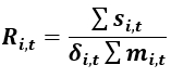
Our model estimates two observable outcomes of changes to state-level prevailing wage laws. The first of these is the quality-adjusted cost of road construction. Thus, our variable of interest is state-level spending, per dollar of road mile rated acceptable by the Federal Highway Administration. This measure includes both new construction and maintenance spending.
Formally it is:
Quality-adjusted road spending R, in state i, in year t, is a sum of spending across all highway/roadway types, s, in state i, in year t. We divide this spending by the sum of road miles, m, in state i, in year t, times the share rated acceptable, δ, for all roads. This is a quality-adjusted, cost-per-mile measure of construction and maintenance.
This measure is designed as a relatively straightforward approximation of cost per mile of maintenance and construction. Annual variation in spending on roads from traditional dedicated funds varies by state. Also, state general funds are often tapped for road construction and maintenance. Another source of annual variation is bonding of larger road projects. A bonding cycle and construction exhibit significant variability. Road spending is not a deterministic fiscal outcome as, say, the result of an excise tax only on gasoline is.
The lengths of available roads also vary significantly. States regularly build new roads and retire others. Municipalities regularly take control of private roads. Over our sample period the largest annual change of road miles in a state was a decline of over 3,500. There was also substantial variation in quality, with the largest annual change of the national mean being two nearly 6% declines in quality.
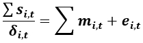
A potential issue in this specification is the value of including the road quality measure. Federal road quality measures are likely endogenous to previous and current levels of spending. Lagged “poor” ratings may incent higher levels of state spending, thus displaying a negative sign. Contemporaneous rankings may be positively correlated with current spending. Our primary concern is that low rankings may suggest states are spending too little to maintain roadways, and if omitted, may bias the effect of prevailing wage legislation and other coefficients.
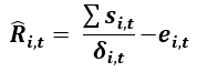
Treating the quality ratings as endogenous means they must either appear in the dependent variable, as proposed here, or be instrumented in a first stage estimation. We focus on the first approach through the remainder of this paper. However, we also estimated a first-stage dependent variable where the state and local spending per road mile was regressed on the federal quality measure. Such that:
so,
This measure yielded results that were statistically identical. The point estimates of the Ȓi,t estimates were marginally higher (1.5 log points) than the Ȓ i,t estimates. We report the more conservative point estimates and prefer the dependent variable Ri,t viewing it as a more direct adjustment of the variable of interest (cost per mile of well-maintained roads) than is Ȓi,t; though the empirical interpretations of both are effectively identical.
Our second model tests the labor share of heavy civil engineering and construction, or formally, total wages and salaries in this sector, divided by total state spending on road construction. This ratio is simply described as Li,t, the labor share of road construction in state i, in year t.
The cost variable R relies solely on data from the same source, without the potential for meaningful miscounting of values due to spending flows to non-construction activities. The labor share variable, L, introduces more risk of dependent variable error since some share of heavy civil engineering and construction employment is spent on non-road construction projects. While our reported labor share estimates in Table 2 fall within reported levels, this is a weakness in the structure of the data we cannot resolve. We will discuss it in more detail in the results and summary sections.[*]
This offers two general specifications:
and
The dependent variables are state and year fixed effects (a), with a prevailing wage dummy PW, in state i and year t, and a matrix X, of explanatory variables and a white noise error term. The values a, ρ and matrix B are to be estimated. This is a standard two-way, fixed-effect model.
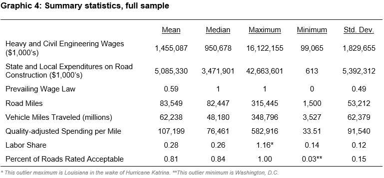
The data we employ are from the Bureau of Economic Analysis, the Bureau of Transportation Statistics and the Federal Highway Administration. Construction worker incomes, as defined by the BEA, are placed into real terms using the Consumer Price Index, All Urban Consumers. Overall road spending is deflated using the Producer Price Index, Streets & Highways. Summary statistics appear in Graphic 4.
There are a few considerations that affect the econometrics of this. In September 2005, President Bush suspended the Davis-Bacon Act, the federal prevailing wage law, for four Gulf Coast states (Alabama, Florida, Louisiana and Mississippi) due to Hurricane Katrina (see Olam and Stamper, 2006). This occurred for less than 60 days. This period is both too brief and too clouded by other factors to provide an identification strategy. However, we did construct a Hurricane Katrina dummy (labeled PW Suspension) for those states in 2005 and included it in full models for each of our dependent variables.
A second concern is the treatment of prevailing wage legislation as a discrete dummy variable. There are states with no state-level prevailing wage laws, and most states with such a law have some minimum applicable cost threshold. For example, California Labor Code Article 2, Sect. 1771 states:
Except for public works projects of one thousand dollars ($1,000) or less, not less than the general prevailing rate of per diem wages for work of a similar character in the locality in which the public work is performed[30] [. . .]
Maryland, which also possesses an active prevailing wage law, has a much higher applicability threshold.
The Prevailing Wage law applies to a public work project including school construction where the contract value is $250,000 or greater and (1) the State or an instrumentality of the State is the contracting body and there is any State funding for the project; (2) a political subdivision is the contracting body and 25% or more of the money used for the construction is State money; or (3) a political subdivision is the contracting body for the construction of an elementary or secondary school and 25% or more of the money used is State money.[31]
The $1,000 threshold in California is sufficiently low that its prevailing wage law functions no differently from laws without thresholds, such as exists in Illinois, Nebraska, New York and Texas, where all government-funded projects apply prevailing wage. We are concerned with the heterogeneity of the dummy and find no effective way to ascertain the size distribution of projects. These contracts are led by state and local governments, and they are made available sporadically across municipal, county, special and state government websites. There is no centralized repository of these data.
Including a small sample dummy variable introduces significant collinearity in our two-way, fixed-effects model. So, in order to test for a role in heterogeneous prevailing wage treatment, we reduce the sample of states. In this case, we provide two ranges to test. We simply omit from our test any state with a minimum prevailing wage contract threshold of $100,000 or less. We do this again based on a threshold of $1,000,000 or less in a state’s legislation. This effectively removes all states with thresholds from our sample. This resulted in the sample size declining from the 48 conterminous states to 35 and then 29 states, respectively.
We omitted Washington, D.C., from the model of roadway costs because its roads have a quality rating that seems unrealistically low. We surmise this is due to factors related to sampling or characteristics, not necessarily related to maintenance issues. This omission significantly reduces the estimated effect of prevailing wage, since Washington, D.C., a prevailing wage jurisdiction, has such high costs per quality-adjusted mile. Not knowing if this is an irrelevant artifact of the data collection or actual data generation process leads us to omit this cross section.
An optimal modeling approach would be a spare treatment model, with both state and year fixed effects; the traditional two-way, fixed effect. Because we have no data preceding the passage of the Davis-Bacon Act, we are unable to evaluate pre-trends that would help us identify this estimation on all our data. However, as noted above, the prevailing wage literature argues against a strong identification problem in a traditional panel, versus difference-in-difference setting.[32] We believe this remains substantially correct.
However, there are reasonable cost elements that should be addressed with controls. The most obvious of these are traffic differentials, which could be included as a value per vehicle miles traveled. Likewise, cost differences include the effect of a federal share of road miles in a state. This fact bolsters the argument against including the District of Columbia in this estimate, since the entirety of that system is federal.
We also aim to have a fuller modeling of annual cost variation. In one version of our estimate, we add to the model a linear time trend, a recession dummy variable and a single series of total U.S. real road construction spending by year. We explain these results more fully in the results section.
Spatial autocorrelation is a concern. We address that problem a priori through the method recommended by Pesaran.[33] However, road work also has network characteristics that warrant direct modeling. The rationale for this is that some roadway funding may include interstate construction, modification or maintenance between two states that is federally funded for both states. The data generating process here is cross-border construction through agreements, such as the Lewis and Clark Bridge between Indiana and Kentucky. Thus, the spatially weighted dependent variable is appropriate, and we use a direct, local spillovers, specification model of the type recommended by LeSage.[34] For this estimation we construct a first-order, contiguity matrix,  , which provides a spatially weighted value of adjacent state road construction spending. The interpretation of these results will be discussed more fully in the results section.
These considerations add significantly to the parameters of our base model. We offer four specifications for each dependent variable. We vary the sample from the full 48 conterminous states to the 35 and 29 states (eliminating the high threshold states), and the six-state sample of those whose prevailing wage legislation changed over the period of study. We estimate the natural log of the dependent variable for ease of interpretation, noting that the labor share is expressed as a share [1,100].
[*] The Vermont Legislative Joint Fiscal Office (2014) reported labor cost shares of 20% to 50% from testimony surrounding the prevailing wage legislation. Rosaen (2013) noted labor share as 25% and 30% in his study, citing earlier work, and in a critique of that work, Phillips (2013) reported labor share estimates of 23% (wages and benefits) for prevailing wage affected employees in all construction. These are germane to our analysis, solely because they frame the size of the potential error. We report the mean labor share of 28% and median of 26%. This is income (including some benefits) for all workers (whether or not they are subject to prevailing wage laws). This provides us comfort that our labor share is reasonably close, and that unusual variation in the share of heavy and civil engineering income spent in a state is random.